6.3: A Confidence Interval for a Population Standard Deviation Unknown, Small Sample Case

In practice, we rarely know the population standard deviation. In earlier problems we have encountered, when the sample size was large, this did not present a problem. They used the sample standard deviation \(s\) as an estimate for \(\sigma\) and proceeded as before to calculate a confidence interval with close enough results. For example, this is what we did in Example 6.2.4. The point estimate for the standard deviation, \(s\), was substituted in the formula for the confidence interval for the population standard deviation. In this case, the 120 observations were well above the suggested 100 observations to eliminate any bias from a small sample. However, statisticians ran into problems when the sample size was small. A small sample size caused inaccuracies in the confidence interval.

William S. Goset (1876–1937) of the Guinness brewery in Dublin, Ireland ran into this problem. His experiments with hops and barley produced very few samples. Just replacing \(\sigma\) with \(s\) did not produce accurate results when he tried to calculate a confidence interval. He realized that he could not use a normal distribution for the calculation; he found that the actual distribution depends on the sample size. This problem led him to "discover" what is called the Student's t-distribution. The name comes from the fact that Gosset wrote under the pen name "A Student."

Some statisticians used the normal distribution approximation for large sample sizes and used the Student's t-distribution only for sample sizes of at most 30 observations, but the two distributions only become interchangeable once \(n\) = 100 or more.

If you draw a simple random sample of size \(n\) from a population with mean \(\mu\) and unknown population standard deviation \(\sigma\) and calculate the t-score \(t=\frac{\overline{x}-\mu}{\left(\frac{s}{\sqrt{n}}\right)}\), then the t-scores follow a Student's t-distribution with \(n - 1\) degrees of freedom. The t-score has the same interpretation as the z-score. It measures how far in standard deviation units \(\overline x\) is from its mean \(\mu\). For each sample size \(n\), there is a different Student's t-distribution.

The degrees of freedom (df), \(n - 1\), come from the calculation of the sample standard deviation \(s\). Remember when we first calculated a sample standard deviation we divided the sum of the squared deviations by \(n - 1\), but we used \(n\) deviations to calculate \(s\). Because the sum of the deviations is zero, we can find the last deviation once we know the other \(n - 1\) deviations. The other \(n - 1\) deviations can change or vary freely. We call the number \(n - 1\) the degrees of freedom (df) in recognition that one is lost in the calculations. The effect of losing a degree of freedom is that the t-value increases and the confidence interval increases in width.

Properties of the Student's t-Distribution

• The graph for the Student's t-distribution is similar to the standard normal curve and at infinite degrees of freedom it is the normal distribution. You can confirm this by reading the bottom line at infinite degrees of freedom for a familiar level of confidence, e.g. at column 0.05, 95% level of confidence, we find the t-value of 1.96 at infinite degrees of freedom.
• The mean for the Student's t-distribution is zero and the distribution is symmetric about zero, again like the standard normal distribution.
• The Student's t-distribution has more probability in its tails than the standard normal distribution because the spread of the t-distribution is greater than the spread of the standard normal. So the graph of the Student's t-distribution will be thicker in the tails and shorter in the center than the graph of the standard normal distribution.
• The exact shape of the Student's t-distribution depends on the degrees of freedom. As the degrees of freedom increases, the graph of Student's t-distribution becomes more like the graph of the standard normal distribution.
• The underlying population of individual observations is assumed to be normally distributed with unknown population mean \(\mu\) and unknown population standard deviation \(\sigma\). This assumption comes from the central limit theorem because the individual observations in this case are the \(\overline x\)s of the sampling distribution. The size of the underlying population is generally not relevant unless it is very small. If it is normal then the assumption is met and doesn't need discussion.

A probability table for the Student's t-distribution (see Appendix A) is used to identify t-values at various commonly-used levels of confidence. The table gives t-scores that correspond to the confidence level (column) and degrees of freedom (row). Notice that at the bottom the table will show the t-value for infinite degrees of freedom. Mathematically, as the degrees of freedom increase, the \(t\) distribution approaches the standard normal distribution. You can find familiar z-values by looking in the relevant alpha column and reading value in the last row.

A Student's t table (see Appendix A) gives t-scores given the degrees of freedom and either a specified level of confidence or the right-tailed probability (depending on which row across the top you are using).

The Student's t-distribution has one of the most desirable properties of the normal: it is symmetrical. What the Student's t-distribution does is spread out the horizontal axis so it takes a larger number of standard deviations to capture the same amount of probability. In reality there are an infinite number of Student's t-distributions, one for each df. As the sample size increases, the Student's t-distribution become more and more like the normal distribution. When the sample size reaches 100 the normal distribution is usually substituted for the Student's t because they are so much alike. This relationship between the Student's t-distribution and the normal distribution is shown in Figure \(\PageIndex{1}\).

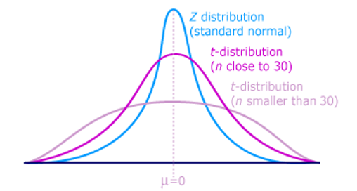
Figure \(\PageIndex{1}\)

Restating the formula for a confidence interval for the mean for cases when the sample size is smaller than 100 and we do not know the population standard deviation, \(\sigma\):

\[\overline{x}-t_{\frac{\alpha}{2}, df}\left(\frac{s}{\sqrt{n}}\right) \leq \mu \leq \overline{x}+t_{\frac{\alpha}{2}, df}\left(\frac{s}{\sqrt{n}}\right)\nonumber\]

Here the point estimate of the population standard deviation, \(s\) has been substituted for the population standard deviation, \(\sigma\), and \(t_{\frac{\alpha}{2}, df}\) has been substituted for \(z_{\frac{\alpha}{2}}\). The notation for df is placed in the general formula in recognition that there are many Student t-distributions, one for each df. For this type of problem, the degrees of freedom is \(df = n - 1\), where \(n\) is the sample size. To look up a probability in the Student's t-table we have to know the degrees of freedom in the problem.

Example \(\PageIndex{1}\)

The average earnings per share (EPS) for 10 industrial stocks randomly selected from those listed on the Dow-Jones Industrial Average was found to be \(\overline x = 1.85\) with a standard deviation of \(s=0.395\). Calculate a 99% confidence interval for the average EPS of all the industrials listed on the Dow Jones.

\[\overline{x}-t_{\frac{\alpha}{2}, df}\left(\frac{s}{\sqrt{n}}\right) \leq \mu \leq \overline{x}+t_{\frac{\alpha}{2}, df}\left(\frac{s}{\sqrt{n}}\right)\nonumber\]

Answer

In this case, we will use the Student’s t-distribution because we do not know the population standard deviation and the sample is small, less than 100.

To find the appropriate t-value requires two pieces of information: the level of confidence desired and the degrees of freedom. The question asked for a 99% confidence level. The tails, thus, need to have .005 probability each, \(\alpha/2\). The degrees of freedom for this type of problem is \(n - 1= 9\).

From the Student’s t-table, at the row marked 9 and column marked for \(\alpha = .005\), is the number of standard deviations to capture 99% of the probability in the t-distribution, and it is 3.250. Remembering that the Student’s \(t\) is symmetrical, this t-value is both plus or minus - appearing on each side of the mean in the distribution.

Inserting these values into the formula gives the result.

\[\mu=\overline{x} \pm t_{.005, 9} \frac{s}{\sqrt{n}}=1.85 \pm 3.250 \frac{0.395}{\sqrt{10}}=1.85 \pm 0.406\nonumber\]

\[1.44 \leq \mu \leq 2.26\nonumber\]

We can interpret this CI by saying: With 99% confidence, the average EPS of all the industries listed on DJIA is between $1.44 and $2.26.

Exercise \(\PageIndex{1}\)

You do a study of hypnotherapy to determine how effective it is in increasing the number of hours of sleep subjects get each night. You measure hours of sleep for 12 subjects with the following results. Construct a 95% confidence interval for the mean number of hours slept for the population (assumed normal) from which you took the data.

8.2; 9.1; 7.7; 8.6; 6.9; 11.2; 10.1; 9.9; 8.9; 9.2; 7.5; 10.5