
6.2: A Confidence Interval for a Population Standard Deviation, Known or Large Sample Size
- Page ID
- 79040
A confidence interval for a population mean with a known population standard deviation is based on the conclusion of the Central Limit Theorem that the sampling distribution of the sample means follow an approximately normal distribution.
Calculating the Confidence Interval
Consider the standardizing formula for the sampling distribution developed in the discussion of the Central Limit Theorem:
\[z_{1}=\frac{\overline{x}-\mu_{\overline{x}}}{\sigma_{\overline{x}}}=\frac{\overline{x}-\mu}{\sigma / \sqrt{n}}\nonumber\]
Notice that \(\mu\) is substituted for \(\mu_{\overline{x}}\) because we know that the expected value of \(\mu_{\overline{x}}\) is \(\mu\) from the Central Limit Theorem and \(\sigma_{\overline{x}}\) is replaced with \(\sigma / \sqrt{n}\), also from the Central Limit Theorem.
In this formula we know \(\overline x\), \(\sigma_{\overline{x}}\) and \(n\), the sample size. (In actuality we do not know the population standard deviation, but we do have a point estimate for it, \(s\), from the sample we took. More on this later.) What we do not know is \(\mu\) or \(z_1\). We can solve for either one of these in terms of the other. Solving for \(\mu\) in terms of \(z_1\) gives:
\[\mu=\overline{x} \pm z_{1} {\sigma} / \sqrt{n}\nonumber\]
Remembering that the Central Limit Theorem tells us that the distribution of the \(\overline x\)'s, the sampling distribution for means, is normal, and that the normal distribution is symmetrical, we can rearrange terms thus:
\[\overline{x}-z_\frac{\alpha}{2}(\sigma / \sqrt{n}) \leq \mu \leq \overline{x}+z_\frac{\alpha}{2}(\sigma / \sqrt{n})\nonumber\]
This is the formula for a confidence interval for the mean of a population.
Notice that \(z_\frac{\alpha}{2}\) has been substituted for \(z_1\) in this equation. This is where a choice must be made by the statistician. The analyst must decide the level of confidence they wish to impose on the confidence interval. \(\alpha\) is the probability that the interval will not contain the true population mean. The confidence level is defined as \((1-\alpha)\). \(z_\frac{\alpha}{2}\) is the number of standard deviations \(\overline x\) lies from the mean with a certain probability. If we chose \(z = 1.96\) we are asking for the 95% confidence interval because we are setting the probability that the true mean lies within the range at 0.95. If we set \(z\) at 1.645 we are asking for the 90% confidence interval because we have set the probability at 0.90. These numbers can be verified by consulting the \(z\)-table (see Appendix A). Divide either (1-0.95) or (1-0.90) in half and find that probability inside the body of the table. Then read on the corresponding top and left margins the number of standard deviations it takes to get this level of probability.
In reality, we can set whatever level of confidence we desire simply by changing the \(z_\frac{\alpha}{2}\) value in the formula. It is the analyst's choice. Convention in business research and most social sciences sets confidence intervals at either 90, 95, or 99 percent levels. Levels less than 90% are considered of little value. The level of confidence of a particular interval estimate is equal to \((1-\alpha)\).
A good way to see the development of a confidence interval is to graphically depict the solution to a problem requesting a confidence interval. This is presented in the figure below for the example in the introduction concerning the number of downloads from iTunes. That case was for a 95% confidence interval, but other levels of confidence could have just as easily been chosen depending on the need of the analyst. However, the level of confidence MUST be pre-set and not subject to revision as a result of the calculations.
Figure \(\PageIndex{1}\)
For this example, let's say we know that the actual population mean number of iTunes downloads is 2.1. The true population mean falls within the range of the 95% confidence interval. There is absolutely nothing to guarantee that this will happen. Further, if the true mean falls outside of the interval we will never know it. We must always remember that we will never ever know the true mean. Statistics simply allows us, with a given level of probability (confidence), to say that the true mean is within the range calculated.
Changing the Confidence Level or Sample Size
Here again is the formula for a confidence interval for an unknown population mean assuming we know the population standard deviation:
\[\overline{x}-z_\frac{\alpha}{2}(\sigma / \sqrt{n}) \leq \mu \leq \overline{x}+z_\frac{\alpha}{2}(\sigma / \sqrt{n})\nonumber\]
It is clear that the confidence interval is driven by two things, the chosen level of confidence, \(z_\frac{\alpha}{2}\), and the standard deviation of the sampling distribution. The standard deviation of the sampling distribution is further affected by two things, the standard deviation of the population and the sample size we chose for our data. Here we wish to examine the effects of each of the choices we have made on the calculated confidence interval, the confidence level and the sample size.
For a moment we should ask just what we desire in a confidence interval. Our goal was to estimate the population mean from a sample. We have forsaken the hope that we will ever find the true population mean, and population standard deviation for that matter, for any case except where we have an extremely small population and the cost of gathering the data of interest is very small. In all other cases we must rely on samples. With the Central Limit Theorem we have the tools to provide a meaningful confidence interval with a given level of confidence, meaning a known probability of being wrong. By meaningful confidence interval we mean one that is useful. Imagine that you are asked for a confidence interval for the ages of your classmates. You have taken a sample and find a mean of 19.8 years. You wish to be very confident so you report an interval between 9.8 years and 29.8 years. This interval would certainly contain the true population mean and have a very high confidence level. However, it hardly qualifies as meaningful. The very best confidence interval is narrow while having high confidence. There is a natural tension between these two goals. The higher the level of confidence, the wider the confidence interval as the case of the students' ages above. We can see this tension in the equation for the confidence interval.
\[\mu=\overline{x} \pm z_{\alpha}\left(\frac{\sigma}{\sqrt{n}}\right)\nonumber\]
The confidence interval widens as confidence level increases, because \(z_\alpha\) will become larger. Sample size also plays an important role in the width of the confidence interval. Notice that the sample size, \(n\), shows up in the denominator of the standard deviation of the sampling distribution. Therefore, as the sample size increases, the standard deviation of the sampling distribution decreases, making the confidence interval narrower. Again, we see the importance of having large samples for our analysis here, although we then face a second constraint, the cost of gathering more data.
Calculating the Confidence Interval: An Alternative Approach
Another way to approach confidence intervals is through the use of something called the error bound. The error bound - also known as the margin of error - gets its name from the recognition that it provides the boundary of the interval derived from the standard error of the sampling distribution. In the equations above it is seen that the interval is simply the estimated mean, sample mean, plus or minus something. That something is the error bound and is driven by the probability we desire to maintain in our estimate, \(z_\alpha\), times the standard deviation of the sampling distribution. The error bound for a mean is given the name, error bound mean, or \(EBM\).
To construct a confidence interval for a single unknown population mean \(\mu\), where the population standard deviation is known, we need \(\overline x\) as an estimate for \(\mu\) and we need the margin of error. Here, the margin of error \((EBM)\) is the error bound for a population mean. The sample mean \(\overline x\) is the point estimate of the unknown population mean \(\mu\).
The confidence interval estimate will have the form:
[point estimate - error bound, point estimate + error bound] or, in symbols, \([\overline{x}-E B M, \overline{x}+E B M]\)
The mathematical formula for this confidence interval is:
\(\overline{x}-z_\frac{\alpha}{2}(\sigma / \sqrt{n}) \leq \mu \leq \overline{x}+z_\frac{\alpha}{2}(\sigma / \sqrt{n})\)
The margin of error depends in part on the confidence level (abbreviated CL). The confidence level is often considered the probability that the calculated confidence interval estimate will contain the true population parameter. However, it is more accurate to state that the confidence level is the percent of confidence intervals that contain the true population parameter when repeated samples are taken. Most often, it is the choice of the person constructing the confidence interval to choose a confidence level of 90% or higher because that person wants to be reasonably certain of his or her conclusions.
There is another probability called alpha (\(\alpha\)). \(\alpha\) is the probability that the interval does not contain the unknown population parameter. Mathematically, \(1 - \alpha = CL\).
A confidence interval for a population mean with a known standard deviation is based on the fact that the sampling distribution of the sample means follow an approximately normal distribution. Suppose that our sample has a mean of \(\overline x = 10\), and we have constructed the 90% confidence interval \([5, 15]\) where \(EBM = 5\).
To get a 90% confidence interval, we must include the central 90% of the probability of the normal distribution. If we include the central 90%, we leave out a total of \(\alpha = .10\) in both tails, or 5% in each tail, of the normal distribution.
Figure \(\PageIndex{2}\)
To capture the central 90%, we must go out 1.645 standard deviations on either side of the calculated sample mean. The value 1.645 is the \(z\)-score from a standard normal probability distribution that puts an area of 0.90 in the center, an area of 0.05 in the far left tail, and an area of 0.05 in the far right tail.
It is important that the standard deviation used must be appropriate for the parameter we are estimating, so in this section we need to use the standard deviation that applies to the sampling distribution for means which we studied with the Central Limit Theorem and is, \(\frac{\sigma}{\sqrt{n}}\).
Calculating the Confidence Interval Using EBM
To construct a confidence interval estimate for an unknown population mean, we need data from a random sample. The steps to construct and interpret the confidence interval are:
- Calculate the sample mean \(\overline x\) from the sample data. Remember, in this section we know the population standard deviation \(\sigma\).
- Find the z-score from the standard normal table that corresponds to the confidence level desired.
- Calculate the error bound.
- Construct the confidence interval.
- Write a sentence that interprets the confidence interval in the context of the situation in the problem.
We will first examine each step in more detail, and then illustrate the process with some examples.
Finding the z-score for the Stated Confidence Level
When we know the population standard deviation \(\sigma\), we use a standard normal distribution to calculate the error bound \(EBM\) and construct the confidence interval. We need to find the value of \(z\) that puts an area equal to the confidence level (in decimal form) in the middle of the standard normal distribution \(Z \sim N(0, 1)\).
The confidence level, \(CL\), is the area in the middle of the standard normal distribution. \(CL = 1 – \alpha\), so \(\alpha\) is the area that is split equally between the two tails. Each of the tails contains an area equal to \(\frac{\alpha}{2}\).
The \(z\)-score that has an area to the right of \(\frac{\alpha}{2}\) is denoted by \(z_{\frac{\alpha}{2}}\).
For example, when \(CL = 0.95\), \(\alpha = 0.05\) and \(\frac{\alpha}{2} = 0.025\); we write \(z_{\frac{\alpha}{2}}\) = \(z_{0.025}\). The area to the right of \(z_{0.025}\) is 0.025 and the area to the left of \(z_{0.025}\) is \(1 – 0.025 = 0.975\).
\(z_{\frac{\alpha}{2}} = z_{0.025} = 1.96\), using a standard normal probability table. We will see later that we can use a different probability table, the Student's \(t\)-distribution, for finding the number of standard deviations of commonly used levels of confidence.
Calculating the Error Bound
The error bound formula for an unknown population mean \(\mu\) when the population standard deviation \sigma is known is
- \(E B M=\left(z \frac{\alpha}{2}\right)\left(\frac{\sigma}{\sqrt{n}}\right)\)
Constructing the Confidence Interval
- The confidence interval estimate has the format \((\overline{x}-E B M, \overline{x}+E B M)\) or the formula: \(\overline{x}-z_\frac{\alpha}{2}(\sigma / \sqrt{n}) \leq \mu \leq \overline{x}+z_\frac{\alpha}{2}(\sigma / \sqrt{n})\)
The graph gives a picture of the entire situation.
\(C L+\frac{\alpha}{2}+\frac{\alpha}{2}=C L+\alpha=1\).
Figure \(\PageIndex{3}\)
Example \(\PageIndex{1}\)
Suppose we are interested in the mean scores on an exam. A random sample of 136 scores is taken and gives a sample mean (sample mean score) of 68. In this example we have the unusual knowledge that the population standard deviation is 3 points. (Do not count on knowing the population parameters outside of textbook examples!) Find a confidence interval estimate for the population mean exam score (the mean score on all exams).
Find a 90% confidence interval for the true (population) mean of statistics exam scores.
- Answer
-
To find the confidence interval, you need the sample mean, \(\overline x\), and the \(EBM\).
\(\overline x = 68\)
\(EBM = \left(z_{\frac{\alpha}{2}}\right)\left(\frac{\sigma}{\sqrt{n}}\right)\)
\(\sigma = 3\); \(n = 136\); the confidence level is 90% \((CL = 0.90)\)
\(CL = 0.90\) so \(\alpha = 1 – CL = 1 – 0.90 = 0.10\)
\(\frac{\alpha}{2}=0.05, z_{\frac{\alpha}{2}}=z_{0.05}\)
The area to the right of \(z_{0.05}\) is \(0.05\) and the area to the left of \(z_{0.05}\) is \(1 – 0.05 = 0.95\).
\(z_{\frac{\alpha}{2}}=z_{0.05}=1.645\)
Because the common levels of confidence in the social sciences are 90%, 95% and 99%, it will not be long until you become familiar with the numbers 1.645, 1.96, and 2.576.
\(E B M=(1.645)\left(\frac{3}{\sqrt{136}}\right)=0.423\)
\(\overline{x}-E B M=68-0.423=67.577\)
\(\overline{x}+E B M=68-0.423=68.423\)
The 90% confidence interval is [67.577, 68.423].
Interpretation: We estimate with 90% confidence that the true population mean exam score for all statistics students is between 67.58 and 68.42.
Example \(\PageIndex{2}\)
Suppose we change the original problem in Example \(\PageIndex{1}\) by using a 95% confidence level. Find a 95% confidence interval for the true (population) mean statistics exam score.
- Answer
-
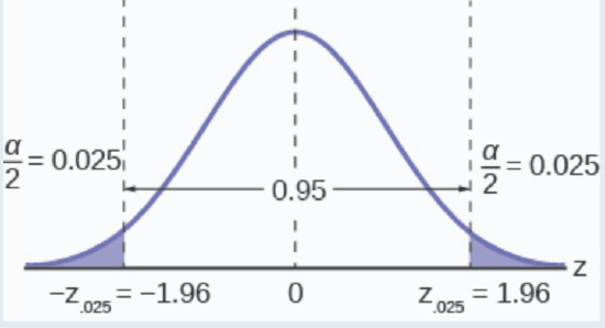 Figure \(\PageIndex{4}\)
\[\mu=\overline{x} \pm z_\frac{\alpha}{2}\left(\frac{\sigma}{\sqrt{n}}\right)\nonumber\]
\[\mu=68 \pm 1.96\left(\frac{3}{\sqrt{136}}\right)\nonumber\]
\[67.50 \leq \mu \leq 68.50\nonumber\]
\(\sigma = 3\); \(n = 36\); the confidence level is 95% (\(CL = 0.95\)).
\(CL = 0.95\) so \(\alpha = 1 – CL = 1 – 0.95 = 0.05\)
\(z_{\frac{\alpha}{2}}=z_{0.025}=1.96\)
Notice that the \(EBM\) is larger and the confidence interval is wider for a 95% confidence level, than it was in the original problem.
Comparing the results
Compared to the 90% confidence interval, the 95% confidence interval is wider. If you look at the graphs, because the area 0.95 is larger than the area 0.90, it makes sense that the 95% confidence interval is wider. To be more confident that the confidence interval actually does contain the true value of the population mean for all statistics exam scores, the confidence interval necessarily needs to be wider. This demonstrates a very important principle of confidence intervals. There is a trade off between the level of confidence and the width of the interval. Our desire is to have a narrow confidence interval, huge wide intervals provide little information that is useful. But we would also like to have a high level of confidence in our interval. This demonstrates that we cannot have both.
Figure \(\PageIndex{5}\)
Summary: Effect of Changing the Confidence Level
- Increasing the confidence level makes the confidence interval wider.
- Decreasing the confidence level makes the confidence interval narrower.
And again here is the formula for a confidence interval for an unknown mean assuming we have the population standard deviation:
\[\overline{x}-z_\frac{\alpha}{2}(\sigma / \sqrt{n}) \leq \mu \leq \overline{x}+z_\frac{\alpha}{2}(\sigma / \sqrt{n})\nonumber\]
The standard deviation of the sampling distribution was provided by the Central Limit Theorem as \(\sigma / \sqrt{n}\). While we infrequently get to choose the sample size it plays an important role in the confidence interval. Because the sample size is in the denominator of the equation, as \(n\) increases it causes the standard deviation of the sampling distribution to decrease and thus the width of the confidence interval to decrease. We have met this before as we reviewed the effects of sample size on the Central Limit Theorem. There we saw that as \(n\) increases the sampling distribution narrows.
Example \(\PageIndex{3}\)
Suppose we change the original problem in Example \(\PageIndex{1}\) once again to see what happens to the confidence interval if the sample size is changed.
Leave everything the same except the sample size. Use the original 90% confidence level. What happens to the confidence interval if we increase the sample size and use \(n = 200\) instead of \(n = 136\)? What happens if we decrease the sample size to \(n = 115\) instead of \(n = 136\)?
- Answer
-
Solution A
\(\mu=\overline{x} \pm z_\frac{\alpha}{2}\left(\frac{\sigma}{\sqrt{n}}\right)\)
\(\mu=68 \pm 1.645\left(\frac{3}{\sqrt{200}}\right)\)
\(67.65 \leq \mu \leq 68.35\)
If we increase the sample size \(n\) to 200, we decrease the width of the confidence interval relative to the original sample size of 136 observations.
- Answer
-
Solution B
\(\mu=\overline{x} \pm z_\frac{\alpha}{2}\left(\frac{\sigma}{\sqrt{n}}\right)\)
\(\mu=68 \pm 1.645\left(\frac{3}{\sqrt{115}}\right)\)
\(67.54 \leq \mu \leq 68.46\)
If we decrease the sample size \(n\) to 115, we increase the width of the confidence interval by comparison to the original sample size of 136 observations.
Summary: Effect of Changing the Sample Size
- Increasing the sample size makes the confidence interval narrower.
- Decreasing the sample size makes the confidence interval wider.
We have already seen this effect when we reviewed the effects of changing the size of the sample, \(n\), on the Central Limit Theorem. Before we saw that as the sample size increased the standard deviation of the sampling distribution decreases. This was why we choose the sample mean from a large sample as compared to a small sample, all other things held constant.
Thus far we assumed that we knew the population standard deviation. This will virtually never be the case. We will have the sample standard deviation, \(s\), however. This is a point estimate for the population standard deviation and can be substituted into the formula for confidence intervals for a mean under certain circumstances. We just saw the effect the sample size has on the width of confidence interval and the impact on the sampling distribution for our discussion of the Central Limit Theorem. We can invoke this to substitute the point estimate for the standard deviation if the sample size is large "enough". Simulation studies indicate that 30 observations or more will be sufficient to eliminate any meaningful bias in the estimated confidence interval.
Example \(\PageIndex{4}\)
Spring break can be a very expensive holiday. A sample of 120 students is surveyed, and the average amount spent by students on travel and beverages is $593.84. The sample standard deviation is approximately $369.34.
Construct a 95% confidence interval for the population mean amount of money spent by spring breakers.
- Answer
-
We begin with the confidence interval for a mean. We use the formula for a mean because the random variable is dollars spent and this is a continuous random variable. The point estimate for the population standard deviation, s, has been substituted for the true population standard deviation.
\[\mu=\overline{x} \pm\left[z_{(\mathrm{\alpha} / 2)} \frac{s}{\sqrt{n}}\right]\nonumber\]
Substituting the values into the formula, we have:
\[\mu=593.84 \pm\left[1.96 \frac{369.34}{\sqrt{120}}\right]\nonumber\]
\(z_{(a / 2)}\) is found on the standard normal table by looking up 0.025 in the body of the table and finding the number of standard deviations on the side and top of the table; 1.96. The solution for the interval is thus:
\[\mu=593.84 \pm 66.09=[527.75,659.93]\nonumber\]
\[\$ 527.75 \leq \mu \leq \$ 659.93\nonumber\]