
9.3: Bond Valuations
- Page ID
- 79788

Video - Audio - YouTube (Material for this section starts on slide 29.)
Bonds are normally priced according to the present value of their future cash flows. Bond investors receive the semi-annual interest payments and the repayment of principal. Of course, other factors will always need to be considered such as the credit-worthiness of the issuer. If an issuer runs into trouble, the price of their outstanding bonds will fall because investors will be afraid of default.
The Discounted Cash Flow Model, Repurposed
Wait a minute! We just said that bonds are normally priced according to the present value of their future cash flows. Doesn’t that sound familiar? Yes, it’s the Discounted Cash Flow Model! The predicted bond price equals the present value of the yearly interest income and the present value of the principal repayment when the bond matures. Since bonds pay interest normally every six months, we really should use semi-annual compounding. However, annual compounding is easier to compute and will give you almost the exact same answer. Annual compounding computations are easily done using the present value tables. Of course, spreadsheets make annual compounding and semi-annual compounding calculations very easy. Here is the formula:
Predicted
Bond = PresentValue (InterestIncome) + PresentValue(Principal Repayment)
Price
First, we will learn how to do the calculation manually. We will then demonstrate the spreadsheet bond calculator which not only is much easier but also much more flexible. The manual calculation involves using our old friend, the present value table from chapter 4. That table gives us the present value multipliers for single payments. However, we will add another version of the present value tables to the mix. We could do the calculations using just the chapter 4 present value table. The only problem is that since bonds pay the same fixed amount each year, it would be very tedious to calculate the present value of each and every year. We would have to do 30 multiplications for a 30-year bond! This new present value table allows us to calculate the present value for a series of payments in just one multiplication calculation. That boils down the entire formula to just two multiplication calculations. The formula becomes:
Predicted Annual Present Value Principal Present Value
Bond = Interest * Multiplier for a + Repayment * Multiplier for a
Price Payment Stream of Payments Single Payment
The left side of the formula computes the present value of the fixed annual bond interest payments. The right side of the formula computes the present value of the principal payment we will receive when the bond matures. We are calculating what the future stream of cash flows from the bond are worth to us today, in the present.
You are thoroughly lost, yes? Again, as was the case when we first learned about present value and discounting and the Discounted Cash Flow Model, the words and concepts are very confusing but the calculations are very easy. After we do the calculations, go back over the paragraphs above and it should make more sense.
Let’s look at an example bond. Idaho Power Company is an electrical power utility company serving Idaho and Oregon. As of April 2023, they have a 5.50% bond coming due in 10 years on 1-Apr-2033, with a par value of $1,000. The bond is rated A-. It was priced to yield 4.994%. This yield is close to 5% so we will use 5% for 10 years since the tables only display data for exact percentages and exact years. Here is a snippet of the present value tables:
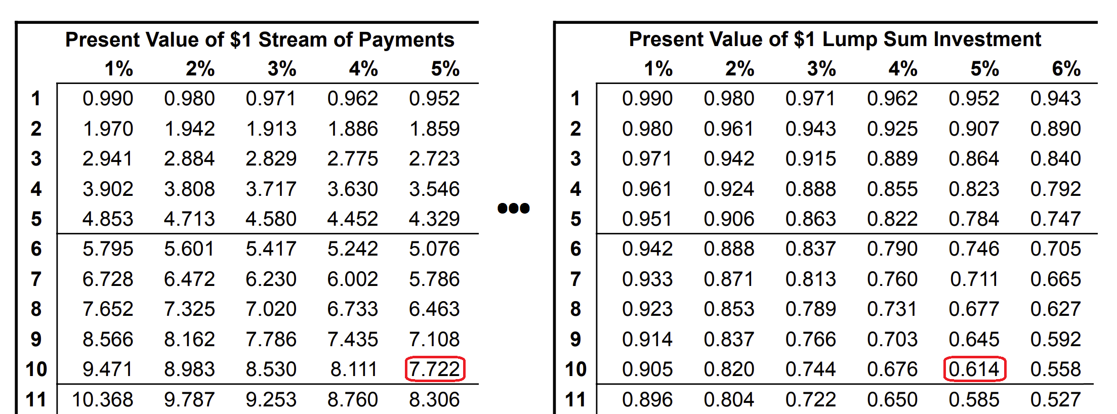
The new table on the left allows us to calculate the present value of a series of payments, also known as a stream of payment or multiple payments. The table on the right is the same table we used in chapter 4. It allows us to calculate the present value of a single, lump sum payment. The annual payment for a $1,000 par value bond paying 5.50% is $55. The formula becomes:
Predicted Annual Present Value Principal Present Value
Bond = Interest * Multiplier for a + Repayment * Multiplier for a
Price Payment Stream of Payments Single Payment
Predicted
Bond Price = $55.00 * 7.722 + $1,000 * 0.614 = $424.71 + $614 ≅ $1,038.71
For the left side of the formula, we use the left table. We go across to 5%, the “priced to yield” value, and then go down to the 10th year. The present value multiplier is 7.722. We multiply the annual interest payment of $55 by the present value multiplier for a stream of payments at 5% for 10 years. That gives us $424.17 on the left side. The ten interest payments we will receive in the future are worth approximately $616.436 today in the present. On the right side, we use the right table. We go across to 5% and down to year 10. The present value multiplier is 0.614. We multiply the principal repayment of $1,000 by the present value multiplier for a single payment at 5% for 10 years. This result is $614; the $1,000 bond principal repayment we will receive in ten years when the bond matures is worth $614 today in the present. Adding together the two values gives us $1,038.71. This is our prediction for the bond price.
How close were we to the actual price? The quoted price on FINRA on April 7th, 2023, was $1,039.49. The bond spreadsheet calculator on the class website gave us $1,039.02 for annual payments and $1,043.02 for semi-annual payments. Pretty close, eh? Why is the prediction using semi-annual payments a bit higher than the annual payments prediction? We are getting paid every six months instead of waiting until the end of the year for the full payment. That makes the present value worth more, not much more, but more.
As mentioned, using the present value tables is impractical. The tables only display present value multipliers for exact years and exact percentages. There is an exponential formula but remember, we promised that you would only need a 99¢ calculator. However, Google Docs is free to use with a Google account. Please view the presentation about the bond spreadsheet calculator and explore the bond spreadsheet calculator itself. Plug in different values and watch how the bond price predictions change.