
4.2: Dividend Discount Models (DDMs)
- Page ID
- 79772

\( \newcommand{\vecs}[1]{\overset { \scriptstyle \rightharpoonup} {\mathbf{#1}} } \)
\( \newcommand{\vecd}[1]{\overset{-\!-\!\rightharpoonup}{\vphantom{a}\smash {#1}}} \)
\( \newcommand{\dsum}{\displaystyle\sum\limits} \)
\( \newcommand{\dint}{\displaystyle\int\limits} \)
\( \newcommand{\dlim}{\displaystyle\lim\limits} \)
\( \newcommand{\id}{\mathrm{id}}\) \( \newcommand{\Span}{\mathrm{span}}\)
( \newcommand{\kernel}{\mathrm{null}\,}\) \( \newcommand{\range}{\mathrm{range}\,}\)
\( \newcommand{\RealPart}{\mathrm{Re}}\) \( \newcommand{\ImaginaryPart}{\mathrm{Im}}\)
\( \newcommand{\Argument}{\mathrm{Arg}}\) \( \newcommand{\norm}[1]{\| #1 \|}\)
\( \newcommand{\inner}[2]{\langle #1, #2 \rangle}\)
\( \newcommand{\Span}{\mathrm{span}}\)
\( \newcommand{\id}{\mathrm{id}}\)
\( \newcommand{\Span}{\mathrm{span}}\)
\( \newcommand{\kernel}{\mathrm{null}\,}\)
\( \newcommand{\range}{\mathrm{range}\,}\)
\( \newcommand{\RealPart}{\mathrm{Re}}\)
\( \newcommand{\ImaginaryPart}{\mathrm{Im}}\)
\( \newcommand{\Argument}{\mathrm{Arg}}\)
\( \newcommand{\norm}[1]{\| #1 \|}\)
\( \newcommand{\inner}[2]{\langle #1, #2 \rangle}\)
\( \newcommand{\Span}{\mathrm{span}}\) \( \newcommand{\AA}{\unicode[.8,0]{x212B}}\)
\( \newcommand{\vectorA}[1]{\vec{#1}} % arrow\)
\( \newcommand{\vectorAt}[1]{\vec{\text{#1}}} % arrow\)
\( \newcommand{\vectorB}[1]{\overset { \scriptstyle \rightharpoonup} {\mathbf{#1}} } \)
\( \newcommand{\vectorC}[1]{\textbf{#1}} \)
\( \newcommand{\vectorD}[1]{\overrightarrow{#1}} \)
\( \newcommand{\vectorDt}[1]{\overrightarrow{\text{#1}}} \)
\( \newcommand{\vectE}[1]{\overset{-\!-\!\rightharpoonup}{\vphantom{a}\smash{\mathbf {#1}}}} \)
\( \newcommand{\vecs}[1]{\overset { \scriptstyle \rightharpoonup} {\mathbf{#1}} } \)
\(\newcommand{\longvect}{\overrightarrow}\)
\( \newcommand{\vecd}[1]{\overset{-\!-\!\rightharpoonup}{\vphantom{a}\smash {#1}}} \)
\(\newcommand{\avec}{\mathbf a}\) \(\newcommand{\bvec}{\mathbf b}\) \(\newcommand{\cvec}{\mathbf c}\) \(\newcommand{\dvec}{\mathbf d}\) \(\newcommand{\dtil}{\widetilde{\mathbf d}}\) \(\newcommand{\evec}{\mathbf e}\) \(\newcommand{\fvec}{\mathbf f}\) \(\newcommand{\nvec}{\mathbf n}\) \(\newcommand{\pvec}{\mathbf p}\) \(\newcommand{\qvec}{\mathbf q}\) \(\newcommand{\svec}{\mathbf s}\) \(\newcommand{\tvec}{\mathbf t}\) \(\newcommand{\uvec}{\mathbf u}\) \(\newcommand{\vvec}{\mathbf v}\) \(\newcommand{\wvec}{\mathbf w}\) \(\newcommand{\xvec}{\mathbf x}\) \(\newcommand{\yvec}{\mathbf y}\) \(\newcommand{\zvec}{\mathbf z}\) \(\newcommand{\rvec}{\mathbf r}\) \(\newcommand{\mvec}{\mathbf m}\) \(\newcommand{\zerovec}{\mathbf 0}\) \(\newcommand{\onevec}{\mathbf 1}\) \(\newcommand{\real}{\mathbb R}\) \(\newcommand{\twovec}[2]{\left[\begin{array}{r}#1 \\ #2 \end{array}\right]}\) \(\newcommand{\ctwovec}[2]{\left[\begin{array}{c}#1 \\ #2 \end{array}\right]}\) \(\newcommand{\threevec}[3]{\left[\begin{array}{r}#1 \\ #2 \\ #3 \end{array}\right]}\) \(\newcommand{\cthreevec}[3]{\left[\begin{array}{c}#1 \\ #2 \\ #3 \end{array}\right]}\) \(\newcommand{\fourvec}[4]{\left[\begin{array}{r}#1 \\ #2 \\ #3 \\ #4 \end{array}\right]}\) \(\newcommand{\cfourvec}[4]{\left[\begin{array}{c}#1 \\ #2 \\ #3 \\ #4 \end{array}\right]}\) \(\newcommand{\fivevec}[5]{\left[\begin{array}{r}#1 \\ #2 \\ #3 \\ #4 \\ #5 \\ \end{array}\right]}\) \(\newcommand{\cfivevec}[5]{\left[\begin{array}{c}#1 \\ #2 \\ #3 \\ #4 \\ #5 \\ \end{array}\right]}\) \(\newcommand{\mattwo}[4]{\left[\begin{array}{rr}#1 \amp #2 \\ #3 \amp #4 \\ \end{array}\right]}\) \(\newcommand{\laspan}[1]{\text{Span}\{#1\}}\) \(\newcommand{\bcal}{\cal B}\) \(\newcommand{\ccal}{\cal C}\) \(\newcommand{\scal}{\cal S}\) \(\newcommand{\wcal}{\cal W}\) \(\newcommand{\ecal}{\cal E}\) \(\newcommand{\coords}[2]{\left\{#1\right\}_{#2}}\) \(\newcommand{\gray}[1]{\color{gray}{#1}}\) \(\newcommand{\lgray}[1]{\color{lightgray}{#1}}\) \(\newcommand{\rank}{\operatorname{rank}}\) \(\newcommand{\row}{\text{Row}}\) \(\newcommand{\col}{\text{Col}}\) \(\renewcommand{\row}{\text{Row}}\) \(\newcommand{\nul}{\text{Nul}}\) \(\newcommand{\var}{\text{Var}}\) \(\newcommand{\corr}{\text{corr}}\) \(\newcommand{\len}[1]{\left|#1\right|}\) \(\newcommand{\bbar}{\overline{\bvec}}\) \(\newcommand{\bhat}{\widehat{\bvec}}\) \(\newcommand{\bperp}{\bvec^\perp}\) \(\newcommand{\xhat}{\widehat{\xvec}}\) \(\newcommand{\vhat}{\widehat{\vvec}}\) \(\newcommand{\uhat}{\widehat{\uvec}}\) \(\newcommand{\what}{\widehat{\wvec}}\) \(\newcommand{\Sighat}{\widehat{\Sigma}}\) \(\newcommand{\lt}{<}\) \(\newcommand{\gt}{>}\) \(\newcommand{\amp}{&}\) \(\definecolor{fillinmathshade}{gray}{0.9}\)One popular group of models of fundamental analysis are the dividend discount models, often abbreviated as DDM or DVM for dividend valuation model. According to the dividend discount models, shares of stock are valued on the basis of the present value of the future dividend streams the stock is projected to produce. Recall that we stated that the value of a stock is based on the present value of its future cash flows. The future cash flows from stocks come from their dividends. Therefore, dividend discount models should be extremely popular, right? During the late 1990’s, investors who adhered to these types of models were considered old fashioned and outdated. But those investors weathered the 2000-2002 downturn very well. Dividends became important again to many investors. “Dividends don’t lie,” is a famous saying. This saying comes from the fact that all the numbers that a company reports on their financial statements could be total fabrications except for one, the dividends. You know the dividends are not a lie because they sent you a check. (Well, actually, they don’t send you a check anymore. The dividends are electronically deposited into your brokerage account but you get the idea.)
The dividend discount models require a discount rate. The discount rate is the required rate of return that we choose to calculate the value of shares of a stock using the dividend discount models. The predicted valuations are very sensitive to our chosen discount rate. Our results will vary widely depending upon our choice. The fact that everyone has a different required rate of return means that different investors will expect and demand different stock prices. Someone might be happy with 6%. Another might expect 10%. A third wants 15%. Mark Twain is reported to have said, “It is the difference of opinion that makes horse races.” This describes the stock market, too.
The term discount rate does cause some uncomfortable looks of confusion from new investors. It does sound a bit strange to many. “Does the discount rate have anything to do with shopping and buying items at a discount?” Uh, no. We will use the terms required rate of return or desired rate of return or expected rate of return. They all mean the same thing as far as the models are concerned.
The Zero Growth Dividend Discount Model
The Zero Growth Dividend Discount Model assumes dividends will continue at a fixed rate indefinitely into the future. It is useful for very mature companies in slow growth or no growth environments. The poster child for the Zero Growth Model is a utility company. Do utility companies grow quickly? In the initial stages of the rapid growth of a city, yes, the local utility will also grow quickly. Think of San Diego County in the 1950’s and 1960’s and San Diego Gas and Electric. However, once the area’s infrastructure is put in place, the utility will grow very slowly, if it grows at all.
The formula for the Zero Growth Model is actually very simple:
                     Annual Dividends

Value of Stock = ———————————————————————

                 Required Rate of Return
For an example, let’s assume that a slow-growth company has been paying $3 of dividends per share for many years and we believe it will continue to do so in the future. If our required rate of return were 6% (0.06), the formula would be:
                     Annual Dividends        $3.00

Value of Stock = ——————————————————————— = ————————— = $50 per share

                 Required Rate of Return      0.06
Does the Zero Growth Model look familiar? It is simply another way to view the Dividend Yield which we calculated in the previous chapter. Recall that the Dividend Yield was calculated as:
                     Annual Dividends

Dividend Yield = ———————————————————————

                  Market Price of Stock
For those of you who enjoy math, note that we simply swapped the Value of Stock with the Market Price of Stock and we swapped the Required Rate of Return with the Dividend Yield. (For those of you who don’t enjoy math, just ignore the previous sentence and hide the Dividend Yield formula.) The take-away is that investors who emphasize the Zero Growth Model are valuing the stock almost exclusively for its dividend yield. What is the current income the stock is generating from its dividends?
For a real-life example, let’s explore Consolidated Edison, symbol ED, the energy utility for New York City and environs. It started its life as the New York Gas Light Company in 1823 and started delivering electricity in 1882. As of February 4, 2025, ED was paying $3.40 in annual dividends and we believe it will continue to pay this dividend into the future. Let’s assume our required rate of return is 8% (0.08). The formula becomes:
                     Annual Dividends       $3.60

Value of Stock = ——————————————————————— = ——————— = $42.50 per share

                 Required Rate of Return     0.08
The current market price as of February 4, 2025, was $94.91 per share. However, the model is stating that we believe the stock is worth only $38.75. Therefore, the model says that the stock is overpriced for our required rate of return. Let’s try a different required rate of return. How about 5%?
                     Annual Dividends       $3.40

Value of Stock = ——————————————————————— = ——————— = $68.00 per share

                 Required Rate of Return     0.05
The model again is stating that we believe the stock is too expensive for us. With a market price of $94.91, the stock is yielding 3.58%. Investors who are happy with a 3.58% required rate of return would believe that ED was correctly priced. Again, the Zero Growth Model works well for stable, income-producing stocks.
Disclaimer: Although they do so very slowly, unlike some other utility companies, Consolidated Edison actually does grow their dividend payments. Therefore, we should really use the next model. However, we simply could not resist showcasing a company that has been in business for 200 years.
The Gordon Growth Dividend Discount Model
The Gordon Growth Dividend Discount Model was named after Myron J. Gordon of the University of Toronto. It is also referred to as the Constant Perpetual Growth Model. This model takes the Zero Growth Model one step further and assumes dividends will continue to grow at a specified rate perpetually into the future. The formula is:
                  ( Annual Dividends * (1 + Dividend Growth Rate) )

Value of Stock = ————————————————————————————————————————————————————

                 ( Required Rate of Return - Dividend Growth Rate )
Compare the formula above with the Zero Growth Model. See how “(1 + Dividend Growth Rate)” has been added to the numerator and “- Dividend Growth Rate” has been added in the denominator. (If you substitute zero for the Dividend Growth Rate, you get the Zero Growth Model. That’s yet another insight for you math-friendly folks.)
For an example, let’s investigate a company that is paying $1 dividend per share. They have been growing their dividend at a constant rate of 5% per year for several years and we believe they will continue to do so going into the future. Our desired rate of return is 10%. Therefore, the formula becomes:
         ( $1 * (1 + 0.05) )      ( $1 * 1.05 )    $1.05

Value = ————————————————————— = ——————————————— = ——————— = $21 per share

           ( 0.10 - 0.05 )            0.05          0.05
The model is telling us that we believe the stock should be valued at $21 per share. This model is good for companies with consistent dividend growth. Companies with consistent dividend growth tend to be large, well-established companies with their roots deep in the economy. Historically, they have been some of the stock market’s best performers over the long term. Remember: Dividends don’t lie!
A note about the arithmetic: We must calculate the numerator and denominator before doing the division. That is why we use the parentheses in the formula. Remember to calculate what is inside the parentheses first.
Let’s look at some real-life examples. Our first is the well-known discount retail chain Target, symbol TGT. As of February 4, 2025, their stock price was $135.60. They are paying $4.48 per year in dividends. Let’s assume that they have been growing their dividend at 8% per year and that our required rate of return is 13%. The formula becomes:
        ( $4.48 * (1 + 0.08) )   ( $4.48 * 1.08 )   $4.8384

Value = —————————————————————— = ———————————————— = ——————— ≈ $96.77

           ( 0.13 - 0.08 )             0.05           0.05
Hmmm. The stock price is $135.60 and our model tells us that we believe it is worth only $96.77 if we desire a 13% rate of return. The model is telling us the stock is overpriced if we require a rate of return of 13%. What if we reduce our expected rate of return to 10%? The only change is to the required rate of return and the formula becomes:
        ( $4.48 * (1 + 0.08) )   ( $4.48 * 1.08 )   $4.8384

Value = —————————————————————— = ———————————————— = ——————— ≈ $241.92

           ( 0.10 - 0.08 )             0.02           0.02
What a big difference! Do you see how sensitive the model is to our required rate of return? By simply changing our required rate of return from 13% to 10%, Target now looks like a bargain. Do you think that Target is a good value? Would you want to own Target? Remember that whenever we research a company, we also need to investigate their competitors, their customers, their suppliers, the industry they are operating in, etc. We do not simply rely on the results from our models. That would be folly.
Our next example is AbbVie, symbol ABBV, a pharmaceutical company that was spun off from Abbott Laboratories several years ago. As of February 4, 2025, the market price was $189.89 and they are currently paying $6.56 in annual dividends. Again, let’s assume the dividends are growing at approximately 8% per year. Let’s again use an expected rate of return of 13%:
        ( $6.56 * (1 + 0.08) )   ( $6.56 * 1.08 )   $7.0848

Value = —————————————————————— = ———————————————— = ——————— ≈ $141.70

           ( 0.13 - 0.08 )             0.05           0.05
At this market price, AbbVie does not look attractive. Let’s again reduce the desired rate of return down to 10%. Remember that the only change is to the required rate of return:
        ( $6.56 * (1 + 0.08) )   ( $6.56 * 1.08 )   $7.0848

Value = —————————————————————— = ———————————————— = ——————— ≈ $354.24

           ( 0.10 - 0.08 )             0.02           0.02
Wow! AbbVie looks like a screaming good deal! However, remember the model is pointing us to companies like AbbVie. As mentioned, this will tilt the odds in our favor. But we now have to spend a whole lotta’ time researching their products, their competitors, customers, suppliers, etc. We can’t rely on the model alone. No, no, no, no, no!
Our third example is Illinois Tool Works. Who or what is Illinois Tool Works? They are one of those companies that have been around for over 100 years and you never hear about them but you are surrounded by their products every day and don’t even know it. Their market price as of February 4, 2025 was $254.80 and they were paying $6.00 in annual dividends. If we assume the same 8% per year dividend growth rate and the same required rate of return of 13%, the formula becomes:
        ( $6.00 * (1 + 0.08) )   ( $6.00 * 1.08 )   $6.48

Value = —————————————————————— = ———————————————— = ——————— ≈ $129.60

           ( 0.13 - 0.08 )             0.05          0.05
Again, at 13%, the model is saying the stock is overpriced. What happens if we again reduce the desired rate of return down to 10%:
        ( $6.00 * (1 + 0.08) )   ( $6.00 * 1.08 )   $6.48

Value = —————————————————————— = ———————————————— = ——————— ≈ $324.00

           ( 0.10 - 0.08 )             0.02          0.02
Maybe we ought to spend more time researching ITW and their competitors. Think of how impressed your friends and family members and colleagues will be when you wax eloquently about large companies important to our economy that they have never heard of.
Now it is your turn to do the calculations. Packaging Corporation of America, symbol PKG, is a company that has been making cardboard boxes … since 1867. As of February 4, 2025, the market price was $210.64. They were paying $5.00 annual dividends and we will assume that they are growing their dividends at 8% per year. Use the model to compute the predicted value at both a 13% and 10% required rate of return. (You should receive $108 for 13% and $270 for 10%.) When people ask me if they should invest in Amazon, I say, “Maybe. But why don’t you research one of the companies that supplies Amazon with the cardboard boxes they use to ship their products?”
Our last example is McDonald’s, symbol MCD, the purveyors of fine foods designed to clog your veins and arteries, encourage certain cancers, and spur Type 2 Diabetes Mellitus. They may even be switching back to pre-1970’s days when beef tallow was the norm. This is a brilliant move that would guarantee many future patients for cardiologists since ingesting beef tallow is a great way to coat your arteries with a substance similar to candle wax. However, there’s a whole lot of money to be made giving people heart disease, strokes, and diabetes. We can then can invest in the companies that then sell them the insulin and the stents! As of February 4, 2025, the market price of McDonald’s was $289.77 and they were paying $7.08 in annual dividends. If we assume a dividend growth rate of 8% and desire a 13% required rate of return, the formula is:
        ( $7.08 * (1 + 0.08) )   ( $7.08 * 1.08 )   $7.6464

Value = —————————————————————— = ———————————————— = ——————— ≈ $152.93

           ( 0.13 - 0.08 )             0.05           0.05
Again, let's try 10%.
        ( $7.08 * (1 + 0.08) )   ( $7.08 * 1.08 )   $7.6464

Value = —————————————————————— = ———————————————— = ——————— ≈ $382.32

           ( 0.10 - 0.08 )             0.02           0.02
Here we see an example of an ethical dilemma that we investors must face from time to time. Here is a company that sells products that are contributing to our most prolific killers: heart disease, cancer, and diabetes. But we aren’t forcing their consumers to buy their products, right? And yet, we all pay for the mess that fast food restaurants create. The profits are privatized; the health costs are socialized. Nothing is perfect, not even capitalism. Would you buy McDonald’s?
Now, after one hypothetical example and five real-life examples, you may be wondering if the Gordon Growth Model is very near and dear to your Humble Author’s heart. You would be right. For all its many limitations, this model is an excellent place to start your research. Please, please, please do not ignore these calculations. They are very easy to do. They will be on exam #2, exam #3, exam #4, and the final exam. You can’t leave BUS-123, Introduction to Investments, without being able to do these simple calculations. It is bad for my self-esteem!
Oh, by the way, you may also be wondering why we simply assumed that the dividend growth rate was 8% for all these companies. Shouldn’t we find the actual dividend growth rates? The answer is, “Yes, of course, we should!” Not only is the model sensitive to our required rate of return, the model is also very sensitive to the dividend growth rate. The recent dividend growth rates of Target, AbbVie, Illinois Tool Works, Packaging Corporation of America, and McDonald’s are all 8.0% or higher. AbbVie is 8.0%, McDonald’s is 8.5%, Target is 8.7%, Packaging Corporation of America is 10.0%, and Illinois Tool Works is 13.1%. All these companies are growing their dividends 8% or higher per year. However, the model does not work if the required rate of return is equal to or less than the dividend growth rate. You get bizarre and anomalous results such as division by zero or negative expected prices. Therefore, we should actually raise our expected rates of returns for all of these companies! According to the model, all these companies are actually better buys than what our initial results were telling us for our required rates of return. Note that these are blue chip companies with long histories of rising dividends. But they are not alone.
The Constant Growth Dividend Discount Model
The Constant Growth Dividend Discount Model assumes dividends will continue to grow at a specified rate for a specified number of years. This model takes the Gordon Growth Model one step further, adding a term to account for constant growth for a set number of years. This is similar to how the Gordon Growth Model evolved from the Zero Growth Model, adding an additional term to account for the consistent growth of dividends. We are going to use a fancy equation editor to display the model. Relax. Before you drop the class, know that we are not going to use this model. We are only showing it to you so you can see how much energy has been put into building these models. The Constant Growth Dividend Discount Model formula is:
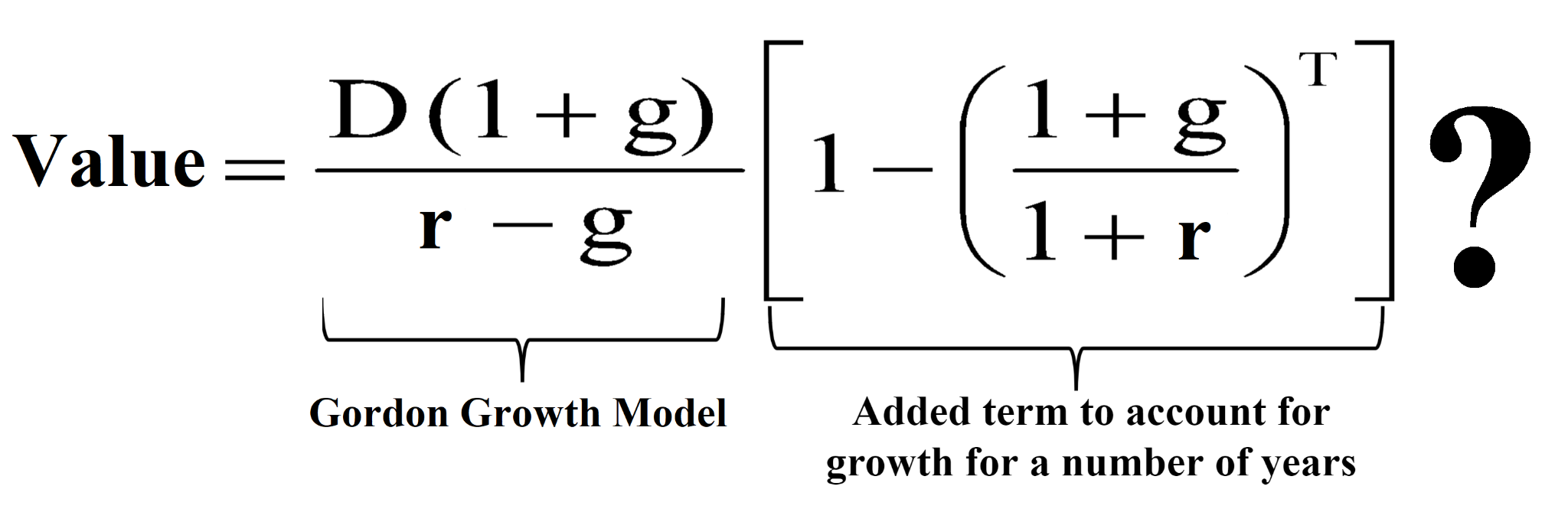
Aye! Scary math stuff! Just gotta’ love those math folks, eh? They use single characters to denote quantities when we normal folks would use an entire descriptive word. The equation is using D as the annual dividend, g as the dividend growth rate, r as the required rate of return, and T as the number of years of growth. The formula computes what we believe the Value of the stock is worth. The ? means that we are afraid that this equation is going to scare students away. Remember we are not going to use this model. Please keep reading. Please don’t drop the class.
Do you see what they have done? The left side of the formula is the Gordon Growth Model that we just studied. To the Gordon Growth Model, they have added another term that takes into account the growth for a set number of years. When using this model, you are asked to estimate just how long the company will be growing their dividends. That is a dubious speculation at best.
Wait. It gets worse.
The Two-Stage Dividend Growth Discount Model
The Two-Stage Dividend Growth Discount Model, also known as the Variable Growth Model, assumes dividends will continue to grow at a specified rate into the future (presumably the fast-growth stage) and then grow at a second (presumably slower growth rate once the company matures). Here it is, Friends:
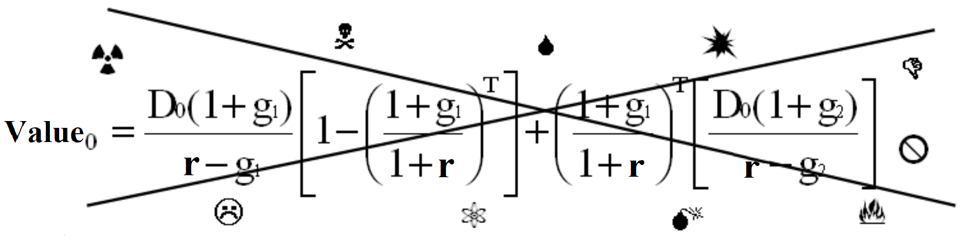
Are you impressed? Well, this model may look very impressive, especially to those who love math, but it has some serious problems. It is very difficult to accurately predict future dividend growth during the initial fast growth stage of a stock. Usually, companies do not pay significant dividends while they are growing quickly because they need the earnings to reinvest in the growth of the company. Again, we show you this model not because we believe it is actually a worthwhile model. We don’t use it and we certainly don’t want you to use it! We show it to you to demonstrate the lengths to which investors have gone to determine the value of companies. Many decades ago in The Intelligent Investor, author Benjamin Graham warned against using overly sophisticated mathematical models to value stocks.
Observations of the Dividend Discount Models
Let’s take a few moments to reflect upon the various Dividend Discount Models that we have covered. One serious issue with the models is that dividend growth rates are very difficult to estimate. With large, well-established companies that have consistently been growing their dividends for a significant period of time, historical growth rates may be useful. But with fast growing companies in new industries, it is almost impossible. However, a more important question arises: How do you use these versions of the models for companies that aren’t paying any dividends? The simple answer is, “You can’t!” If a company is not paying dividends, then the present value of the future stream of no dividends is zero! These models say that a company that does not pay any dividends is worthless. This is obviously not true. The problems of the previous Dividend Discount Models notwithstanding, repeat after me: “The value of a stock is based on the present value of its future cash flows.”
Now, if only there were a model that could value a company that is not paying dividends. Ah, Dear Students, read on. You are all about to become full-fledged Investment Gurus!