
6.5: Life Cycle Costs, Taxes and Finance of Infrastructure
- Page ID
- 21142

For long term rehabilitation investment planning, a life cycle viewpoint is normally used. ‘Life cycle’ in this context generally refers to a planning horizon for investments and not necessarily the obsolescence of some infrastructure. In performing life cycle analysis, you must select an appropriate planning horizon, a discount rate to account for the time value of money, and forecast benefits and costs of the infrastructure over the course of the planning horizon.
Selection of a planning horizon and a discount rate are often organizational choices, so most infrastructure managers need not be concerned with these two inputs. For the US, any project involving federal dollars must use the discount rate chosen by the US Office of Management and Budget (OMB, 2015). In the absence of organizational guidance, an infrastructure manager might use a discount rate reflecting marketplace long term borrowing rates and a planning horizon consistent with the expected useful lifetime of the infrastructure. For example, a planning horizon for a building might be fifty years, while a cellular hub might be ten years.
Even formulation of the short run cost functions discussed earlier can involve life cycle cost analysis to estimate the fixed costs of infrastructure in each period. Infrastructure typically requires an initial large capital expenditure for construction, and this fixed cost is usually annualized to uniform amounts to obtain the fixed costs allocated to any year of operation. The formula for annualization of an initial cost \(P\) to uniform amounts \(U\) over a planning period with n compounding periods at a discount rate \(I\) is (Au, 1992):
\[U=P\left[\frac{i(1+i)^{n}}{(1+i)^{n}-1}\right]\]
Where \(U\) is the uniform annualized amount, \(P\) is the present expenditure, \(i\) is a discount rate and \(n\) is the planning horizon (or technically the number of compounding periods). This process is equivalent to that of assuming a mortgage on the infrastructure component in which the entire construction cost is borrowed at an interest rate of \(i\) and a repayment period of \(n\) years.
Why isn’t the uniform amount simply the value \(P\) divided by the number of payment periods, \(frac{P}{n}\)? The use of a discount rate reflects the ‘time value of money.’ Lenders usually require a return on their lending, so they charge an interest rate. Individuals always prefer receiving money in the present rather than an equivalent amount in the future. The amount of extra required to make a future amount equivalent is a personal discount rate. Organizational discount rates are typically set with reference to the market equilibrium for long term borrowing.
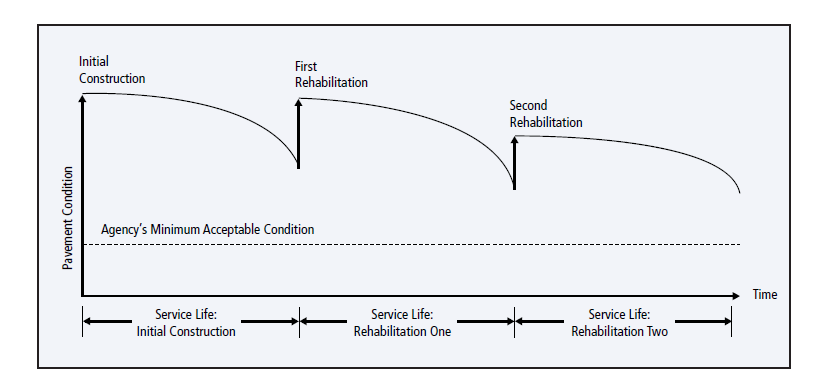
In addition to the initial capital construction expenditure, infrastructure will often have major expenditures associated with rehabilitation. Figure 6.5.1 illustrates this type of rehabilitation. The pavement condition deteriorates during use and weathering until a rehabilitation occurs. The rehabilitations have lower cost than the initial construction and take place over the service lifetime of the pavement. For discussion of methods of estimating such costs, see Hendrickson (2008).
How can these rehabilitation expenses be converted into a uniform annual cost? The most direct means is to find the present value of such costs over the infrastructure lifetime by discounting future costs:
\[P=\sum_{(t=o)}^{n} F_{t}(1+i)^{-t}\]
Where P is present value, t is a time index, n is the planning horizon, Ft is the cost incurred in year t, and i is the discount rate. Uniform costs can then be obtained using Equation 6.5.1.
As a numerical example, suppose the costs illustrated in Figure 6.5.1 are estimated as shown in Table 6.5.1. With a 30-year planning horizon and a 1% discount rate, the life cycle costs (in $ million) would be:
\(\text{P = Initial Construction Cost + Discounted First and Second Rehabilitation + Discounted Maintenance Cost}\)
\[=5+\frac{2}{1.01^{10}}+\frac{1}{1.01^{20}}+\sum_{t=1}^{30} 0.1 * 1.01^{-t}\]
\(= 5 + 1.8 + 0.8 + 2.6 = 10.2\)
For a social cost analysis of the pavement, user costs of roadway delays for construction might be added.
Table 6.5.1: Illustration of Costs for a Life Cycle Cost Analysis.
| Cost COmponent | Year of Occurence | Cost Estimate (Base year $) |
| InitialConstruction | 0 | $ 5 million |
| First Rehabilitation | 10 | $ 2 million |
| Second Rehabilitation | 20 | $ 1 million |
| Annual Maintenance | Each year 1-30 | $ 0.1 million |
Inflation and deflation will affect life cycle cost analysis if current dollars are used for analysis. With inflation, the purchasing value of a unit of currency declines over time; deflation reflects an increase in the value of a currency. Current dollar amounts can be converted to ‘real’ or base year dollar amounts by applying an inflation index adjustment: \(\text(Index_{base year} / Index_t)\) or by discounting using Eq. 6.5.2 and the expected rate of inflation. Different types of infrastructure have their own inflation indexes or a general index such as the gross domestic product index can be used. Life cycle cost estimates are generally made in base year ‘real’ dollars. Financial agreements for payments such as mortgages usually are based upon current dollars. With these mixed dollar amounts, you should apply an inflation calculator to convert to one type of dollar amount.
Discount rates also can be for constant ‘real’ dollars or for current inflated dollars. The relationship is:
\[I' = I + j = ij\]
Where \(I’\) is the annual discount rate including inflation (for current dollar discounting), \(I\) is the real discount rate, and \(j\) is the inflation rate. Readers unfamiliar with these engineering economics calculations can refer to Au (1992) or other textbooks.
For investment decisions, the life cycle costs can be compared to the life cycle benefits in a similar fashion by placing the costs and benefits into present values. In this case, you can examine the net present value of an investment: \( \text(NPV = P_{benefit} – P_{cost})\). With a series of mutually exclusive infrastructure design or rehabilitation options, you might select the one that maximizes this net present value.
Spreadsheet or numerical analysis software is readily available to perform the engineering economics calculations for analyzing life cycle costs. For a spreadsheet, a separate row (or if you prefer a separate column) is used for each period and the costs and benefits recorded. The discounting functions in Equations 6.5.1 and 6.5.2 are usually already available in the software.