
8: Present Value Models
- Page ID
- 12753

\( \newcommand{\vecs}[1]{\overset { \scriptstyle \rightharpoonup} {\mathbf{#1}} } \)
\( \newcommand{\vecd}[1]{\overset{-\!-\!\rightharpoonup}{\vphantom{a}\smash {#1}}} \)
\( \newcommand{\dsum}{\displaystyle\sum\limits} \)
\( \newcommand{\dint}{\displaystyle\int\limits} \)
\( \newcommand{\dlim}{\displaystyle\lim\limits} \)
\( \newcommand{\id}{\mathrm{id}}\) \( \newcommand{\Span}{\mathrm{span}}\)
( \newcommand{\kernel}{\mathrm{null}\,}\) \( \newcommand{\range}{\mathrm{range}\,}\)
\( \newcommand{\RealPart}{\mathrm{Re}}\) \( \newcommand{\ImaginaryPart}{\mathrm{Im}}\)
\( \newcommand{\Argument}{\mathrm{Arg}}\) \( \newcommand{\norm}[1]{\| #1 \|}\)
\( \newcommand{\inner}[2]{\langle #1, #2 \rangle}\)
\( \newcommand{\Span}{\mathrm{span}}\)
\( \newcommand{\id}{\mathrm{id}}\)
\( \newcommand{\Span}{\mathrm{span}}\)
\( \newcommand{\kernel}{\mathrm{null}\,}\)
\( \newcommand{\range}{\mathrm{range}\,}\)
\( \newcommand{\RealPart}{\mathrm{Re}}\)
\( \newcommand{\ImaginaryPart}{\mathrm{Im}}\)
\( \newcommand{\Argument}{\mathrm{Arg}}\)
\( \newcommand{\norm}[1]{\| #1 \|}\)
\( \newcommand{\inner}[2]{\langle #1, #2 \rangle}\)
\( \newcommand{\Span}{\mathrm{span}}\) \( \newcommand{\AA}{\unicode[.8,0]{x212B}}\)
\( \newcommand{\vectorA}[1]{\vec{#1}} % arrow\)
\( \newcommand{\vectorAt}[1]{\vec{\text{#1}}} % arrow\)
\( \newcommand{\vectorB}[1]{\overset { \scriptstyle \rightharpoonup} {\mathbf{#1}} } \)
\( \newcommand{\vectorC}[1]{\textbf{#1}} \)
\( \newcommand{\vectorD}[1]{\overrightarrow{#1}} \)
\( \newcommand{\vectorDt}[1]{\overrightarrow{\text{#1}}} \)
\( \newcommand{\vectE}[1]{\overset{-\!-\!\rightharpoonup}{\vphantom{a}\smash{\mathbf {#1}}}} \)
\( \newcommand{\vecs}[1]{\overset { \scriptstyle \rightharpoonup} {\mathbf{#1}} } \)
\(\newcommand{\longvect}{\overrightarrow}\)
\( \newcommand{\vecd}[1]{\overset{-\!-\!\rightharpoonup}{\vphantom{a}\smash {#1}}} \)
\(\newcommand{\avec}{\mathbf a}\) \(\newcommand{\bvec}{\mathbf b}\) \(\newcommand{\cvec}{\mathbf c}\) \(\newcommand{\dvec}{\mathbf d}\) \(\newcommand{\dtil}{\widetilde{\mathbf d}}\) \(\newcommand{\evec}{\mathbf e}\) \(\newcommand{\fvec}{\mathbf f}\) \(\newcommand{\nvec}{\mathbf n}\) \(\newcommand{\pvec}{\mathbf p}\) \(\newcommand{\qvec}{\mathbf q}\) \(\newcommand{\svec}{\mathbf s}\) \(\newcommand{\tvec}{\mathbf t}\) \(\newcommand{\uvec}{\mathbf u}\) \(\newcommand{\vvec}{\mathbf v}\) \(\newcommand{\wvec}{\mathbf w}\) \(\newcommand{\xvec}{\mathbf x}\) \(\newcommand{\yvec}{\mathbf y}\) \(\newcommand{\zvec}{\mathbf z}\) \(\newcommand{\rvec}{\mathbf r}\) \(\newcommand{\mvec}{\mathbf m}\) \(\newcommand{\zerovec}{\mathbf 0}\) \(\newcommand{\onevec}{\mathbf 1}\) \(\newcommand{\real}{\mathbb R}\) \(\newcommand{\twovec}[2]{\left[\begin{array}{r}#1 \\ #2 \end{array}\right]}\) \(\newcommand{\ctwovec}[2]{\left[\begin{array}{c}#1 \\ #2 \end{array}\right]}\) \(\newcommand{\threevec}[3]{\left[\begin{array}{r}#1 \\ #2 \\ #3 \end{array}\right]}\) \(\newcommand{\cthreevec}[3]{\left[\begin{array}{c}#1 \\ #2 \\ #3 \end{array}\right]}\) \(\newcommand{\fourvec}[4]{\left[\begin{array}{r}#1 \\ #2 \\ #3 \\ #4 \end{array}\right]}\) \(\newcommand{\cfourvec}[4]{\left[\begin{array}{c}#1 \\ #2 \\ #3 \\ #4 \end{array}\right]}\) \(\newcommand{\fivevec}[5]{\left[\begin{array}{r}#1 \\ #2 \\ #3 \\ #4 \\ #5 \\ \end{array}\right]}\) \(\newcommand{\cfivevec}[5]{\left[\begin{array}{c}#1 \\ #2 \\ #3 \\ #4 \\ #5 \\ \end{array}\right]}\) \(\newcommand{\mattwo}[4]{\left[\begin{array}{rr}#1 \amp #2 \\ #3 \amp #4 \\ \end{array}\right]}\) \(\newcommand{\laspan}[1]{\text{Span}\{#1\}}\) \(\newcommand{\bcal}{\cal B}\) \(\newcommand{\ccal}{\cal C}\) \(\newcommand{\scal}{\cal S}\) \(\newcommand{\wcal}{\cal W}\) \(\newcommand{\ecal}{\cal E}\) \(\newcommand{\coords}[2]{\left\{#1\right\}_{#2}}\) \(\newcommand{\gray}[1]{\color{gray}{#1}}\) \(\newcommand{\lgray}[1]{\color{lightgray}{#1}}\) \(\newcommand{\rank}{\operatorname{rank}}\) \(\newcommand{\row}{\text{Row}}\) \(\newcommand{\col}{\text{Col}}\) \(\renewcommand{\row}{\text{Row}}\) \(\newcommand{\nul}{\text{Nul}}\) \(\newcommand{\var}{\text{Var}}\) \(\newcommand{\corr}{\text{corr}}\) \(\newcommand{\len}[1]{\left|#1\right|}\) \(\newcommand{\bbar}{\overline{\bvec}}\) \(\newcommand{\bhat}{\widehat{\bvec}}\) \(\newcommand{\bperp}{\bvec^\perp}\) \(\newcommand{\xhat}{\widehat{\xvec}}\) \(\newcommand{\vhat}{\widehat{\vvec}}\) \(\newcommand{\uhat}{\widehat{\uvec}}\) \(\newcommand{\what}{\widehat{\wvec}}\) \(\newcommand{\Sighat}{\widehat{\Sigma}}\) \(\newcommand{\lt}{<}\) \(\newcommand{\gt}{>}\) \(\newcommand{\amp}{&}\) \(\definecolor{fillinmathshade}{gray}{0.9}\)After completing this chapter, you should be able to: (1) identify the different kinds of present value (PV) models; (2) understand the types of questions different PV models can answer; and (3) construct PV models that represent defending and challenging investments.
To achieve your learning goals, you should complete the following objectives:
- Learn about the different kinds of PV models.
- Learn about the unique questions each kind of PV model can answer.
- Learn how to construct the following PV models:
- net present value (NPV),
- internal rate of return (IRR),
- maximum (minimum) bid (sell),
- annuity equivalent (AE),
- break-even,
- optimal life, and
- payback.
- Learn how to represent the opportunity cost of the defender using its return on equity (ROE) or its return on assets (ROA).
Introduction
Picture yourself traveling across the country driving a luxury car or a tractor. Alternatively, picture yourself pulling a plow with a luxury car or a tractor. While both a luxury car and a tractor can provide transportation and pulling services, they are not equally suited for the two assignments.
One word economists use to describe activities a firm can perform but with unequal efficiency is comparative advantage. Luxury cars are perfectly suited for traveling across country but not for pulling a plow. A tractor is well designed for pulling a plow but not for long-distance travel.
Similarly, there are several different kinds of PV models, but they are designed for answering different kinds of questions. Each model has a comparative advantage for answering a particular kind of question. In what follows we examine some of the most important PV models and the questions they can be used to answer.
Net Present Value Models
In a static (timeless) model, profits describe the difference between costs and returns. In a PV model, an equivalent concept is called the Net Present Value (NPV). The NPV measures the difference in present dollars between cash outflows and cash inflows. NPV models reveal whether the present benefits of an investment outweigh its present costs. The important difference between NPV models and profit calculations is that profits may include non-cash returns and expenses such as increases in inventory and depreciation. The numbers that enter PV models besides the discount rate and the exponents on the discount rate of dollar are cash flow measures where the liquidation value of the investment at the end of its economic life is treated as though it were converted to cash.
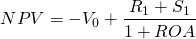
Suppose an investment in a challenger requires an outflow of V0 dollars and generates a positive cash flow of R1 dollars one period later plus the investment’s liquidation value S1. For now, assume that the discount rate, or the rate of exchange between present and future dollars for the defender, is r percent, and represents the opportunity cost of sacrificing the defender to invest in the challenger. To determine if the benefits of this investment outweigh the costs, we find the NPV defined as:
\[ \label{8.1} N P V=-V_{0}+\frac{R_{1}+S_{1}}{(1+r)}\]
Suppose a challenging investment costs $100 and returns R1 = $100 and S1 = $20 in period one while the defending investment could earn r equal to 10%. Then the NPV of this investment would be:
\[N P V=-100+\frac{\$ 100+\$ 20}{1.1}=\$ 9.09 \label{8.2}\]
For this investment, NPV is positive, and the present value of cash benefits outweighs the present value of cash costs. Another way to describe this result is that the challenger earned a higher rate of return than the defender. How much more? The exchange rate for the challenger is ($100 + $20)/$100 = 1.20 compared to $110/$100 = 1.10 for the defender.
But what does it mean to say that the challenger earned a higher rate of return than the defender? An investment is a commitment you make to a project. If the project pays you more than the rate of return on the defender, then the investment’s NPV is positive. In our example the project pays at the rate of 20%. In NPV models, think of the discount rate as the rate earned by the defending investment. And if NPV is positive, the challenger will earn a rate of return higher than could be earned by continuing to invest in the defender.
Of course, investments can be much more complicated than described above. For example, an investment may generate (positive and negative) cash flows for n periods (R1, R2, ⋯, Rn) rather than just one period. Furthermore, most capital assets generate a positive or negative liquidation value (Sn) at the end of its economic life which should be accounted for explicitly.
Using subscripts to indicate the time periods in which the cash flows occur, we write a more complete NPV model as:
\[N P V=-V_{0}+\frac{R_{1}}{(1+r)}+\frac{R_{2}}{(1+r)^{2}}++\frac{R_{n}}{(1+r)^{n}}+\frac{S_{n}}{(1+r)^{n}} \label{8.3}\]
Internal Rate of Return (IRR) Models
Assume that the cash flow represented in Equation \ref{8.3} are largely determined by the market or from other sources of information and are known. But where do we find r, the opportunity cost of capital, the rate of return earned on the defender? The answer is that we set the NPV of the cash flow that describes the defender equal to zero and solve for the discount rate which we then refer to as the defender’s internal rate of return or its IRR. In such a model, the IRR will be equal to the defender’s ROE or its ROA depending on the focus of the PV model. To make clear the distinction between cash flows associated with the challenging and defending investments we adopt the following notation: we superscript cash flow for the challenger with the lowercase letter “c” and cash flow for the defender with the lowercase letter “d”.
\[N P V^{d}=-V_{0}^{d}+\frac{R_{1}^{d}+S_{1}^{d}}{(1+r)} \label{8.4}\]
Now set NPVd equal to zero. Such a PV model in which NPV is set equal to zero is called an Internal Rate of Return (IRR) model, and r is the rate at which dollars are exchanged between time periods for the defender. Because NPV is zero in this model, r is exactly the rate of return earned on the defending investment, the rate at which future dollars earned on the investment are exchanged for present dollars. Finally, the internal rate of return earned on the defender is what is sacrificed to invest in the challenger, and equals the opportunity cost in the NPV model. (The calculation of the defender’s IRR in multi-period models can be much more complex.) To illustrate, we solve for the rate of return earned on the defender or the IRR in the previous model. The IRR equals:
\[r=\frac{R_{1}^{d}}{V_{0}^{d}}-1 \label{8.5}\]
Next substitute the defender’s IRR into the NPV model of the challenger:
\[N P V^{c}=-V_{0}^{c}+\frac{R_{1}^{c}+S_{1}^{c}}{(1+r)} \label{8.6}\]
If the NPV of the challenger is positive, the challenger is preferred to the defender. Why? Because exchanging future dollars for present dollars at the same rate of exchange as the defender leaves the investor with a positive net present value.
Maximum Bid (Minimum Sell) Models
Different kinds of investment questions created the need for different kinds of PV models. The maximum bid and minimum sell models assume r is known and NPV is zero. The models then solve for the purchase price of an investment in a maximum bid price model, or the sale price in a minimum sell price model. In a maximum bid model, the sale price that equates NPV to zero indicates how much the buyer can bid for the investment and still earn the IRR rate r on the defender. Or, from the seller’s perspective, the minimum sell price is the lowest price a seller can accept in exchange for the cash flow stream generated by the investment and still earn the IRR rate r earned on the defender.
To illustrate, begin by assuming that r,
the IRR of the defender, is known as well as the cash flow that can
be earned by the challenger. Now evaluate the challenger by setting
NPV equal to zero and finding the maximum bid (minimum sell) price
 :
:
\[N P V^{c}=-V_{0}^{c}+\frac{R_{1}^{c}+S_{1}^{c}}{(1+r)}=0 \label{8.7}\]
The maximum bid (minimum sell) price is:
\[V_{0}^{c}=\frac{R_{1}^{c}+S_{1}^{c}}{(1+r)} \label{8.8}\]
The Break-even Model
Assume that the investor knows the investment cost ,
its liquidation value  ,
and the IRR of the defender r but doesn’t know the amount
of returns on the challenger
,
and the IRR of the defender r but doesn’t know the amount
of returns on the challenger  that
would be required if the investment were to earn a rate of return
equal to that available on the defender. The firm can find the
amount required to return break-even earnings by setting the NPV
model to zero and solving for R1 as
follows:
that
would be required if the investment were to earn a rate of return
equal to that available on the defender. The firm can find the
amount required to return break-even earnings by setting the NPV
model to zero and solving for R1 as
follows:
\[ \label{8.9} N P V^{c}=-V_{0}^{c}+\frac{R_{1}^{c}+S_{1}^{c}}{(1+r)}=0\]
and the break-even earnings amount is:
\[R_{1}^{c}=(1+r) V_{0}^{c}-S_{1}^{c} \label{8.10}\]
If r were 10%, the liquidation value
were zero, and the initial investment of were
$100, then the break-even return would be $100(1.1) = $110, the
amount the investment would be required to earn in order to
break-even. Break-even here has a specific meaning which is to earn
the defender’s IRR.
The Annuity Equivalent (AE) Model
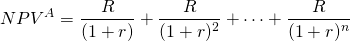
An annuity is a financial product sold by financial institutions. The essence of an annuity is that an individual pays into a fund that is invested and grows until some point in time when the investment is paid back to the investor as a constant stream of payments for a specified period of time. In this book we define a related concept, an annuity equivalent. An annuity equivalent is a constant stream of payments whose present value is equivalent to some other stream of payments that may not be constant. The annuity equivalent model finds an annuity associated with an investment. An annuity is like a time adjusted average. Suppose we wished to find the annuity equivalent associated with the generalized NPV model below:
(8.11)

Now consider an alternative model in which the NPVA is equal to the NPVA in Equation \ref{8.11}:
(8.12)
The value for R in Equation \ref{8.12} is the annuity equivalent cash flow that yields NPVA in Equation \ref{8.11}.
Because annuity equivalents appear in so many contexts, including constant payment loans, retirement benefit payouts, and others, we adopt a notation to describe them. Factoring R in Equation \ref{8.12} we write:
(8.13)

The notation  equals the bracketed expression in Equation \ref{8.13} and stands
for the sum of a uniform series of $1 payments discounted by a rate
of r for n periods. Obviously, there is a direct
correlation between NPVs and annuity equivalents, and both are used
to rank investments.
equals the bracketed expression in Equation \ref{8.13} and stands
for the sum of a uniform series of $1 payments discounted by a rate
of r for n periods. Obviously, there is a direct
correlation between NPVs and annuity equivalents, and both are used
to rank investments.
To illustrate, suppose that NPV were $10,000,
monthly installments were for 5 years, and the discount rate were 3
percent. The AE for this investment is equal to $179.69 and

Optimal Life Models
Optimal life models ask what is the optimal life of this investment? The optimal life model can be written as:
(8.14)

or in continuous time as:
(8.15)
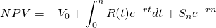
The optimal solution has a specific meaning in the context of the optimal life model. It is that value of n that maximizes the NPV. Formally, the solution employs calculus to optimize the NPV. In the discrete models which are most often employed in practice, the optimal value is found through trial and error or through repeated calculations of alternative values for n.
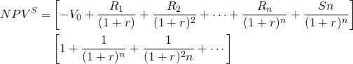
A related optimal life model asks: what is the optimal value of n that maximizes NPV if there are replacements for the investment? In this case, NPVS is the sum of NPVs from individual investments. Such a replacement model is described below:
(8.16)
The Payback Model
While PV models are generally carefully deduced and the data required to solve them is explicit, sometimes decision makers just want a “ball park” estimate of the desirability of a financial strategy. In such cases, decision makers are willing to sacrifice rigor and precision for approximations. When this is the case, the payback model is often employed. To obtain an approximation, it assumes the discount rate in PV models is zero. In other words, the payback model assumes that present and future dollars are valued the same—a very unrealistic assumption. Then the payback model calculates the number of periods required to earn the investment’s present value. The number of periods required to earn the investment’s value is the payback period, the criterion used to rank investments. All cash flow after the payback period is assumed to have no influence on the criterion. To illustrate, n is the payback period in the payback model that follows.
(8.17)

And if periodic cash flows are constant we can express the payback period as:
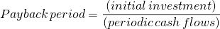
To illustrate, consider an initial outflow of $5,000 with $1,000 cash inflows per month. In this case, the payback period would be 5 months. If the cash inflows were paid annually, then the result would be 5 years. More generally, cash flows will not be equal to one another. If $10,000 is the initial outflow investment, and the cash inflows are $1,000 at year one, $6,000 at year two, $3,000 at year three, and $5,000 at year four, then the payback period would be three years, as the first three years are equal to the initial outflow.
Despite its popularity, the payback model is not recommended for several reasons. Mainly, ignoring the time value of money basically treats an inter temporal investment as though it were a static profit problem. Furthermore, it treats cash flows earned after the payback period as though they were of no worth. In sum, in many respects it inadequately accounts for important elements of the investment problem.
Ranking Investments
Questions PV models answer. It may be helpful to categorize PV models into similar types by recognizing the questions they can answer. The first type answers the question: what is the break-even price such that NPV is zero. Included in this category are maximum bid (minimum sell) models, break-even models, and annuity-equivalent models. A second type of model answers the question: what is they optimal life of the investment. These models find the time period that maximizes NPV. The third type of PV model—and the most popular—are PV models that rank investments. They answer the question: which investment is preferred? The two most popular ranking PV models are the NPV and IRR models. In one survey, about 75% of chief financial officers of large corporations used IRR and NPV models nearly equally (Graham and Harvey, 2001). About 50% used payback models.
The advantage of the NPV model is that we can experiment with several different IRRs to find out how sensitive the NPV of the challenger is to alternative discount rates or IRRs. As we will discover in later chapters, consistency between NPV and IRR rankings exists only under homogeneous measures of size, term, taxes, and other measures.
There are alternative, easier ways of ranking investments such as the payback model. They are not recommended here because they fail to recognize a fundamental property of PV models: dollars in different time periods are valued differently and ignore cash flows after the payback period.
More complicated investment ranking problems. When we described the NPV model, the discount rate was equal to the defender’s IRR. When the firm is considering the adoption of two mutually exclusive investments, then which investment is the defender and which is the challenger is an arbitrary decision. If the capital budgeting decision is to replace an existing investment with one of two mutually exclusive investments, then typically the defender is the investment in place. Then, the investment problem becomes calculating the NPV of the two challenging investments and selecting the one with the greater NPV.
More complicated ranking problems involve replacing a defender with a newer version of the same investment. Such an investment might be when to replace a cohort of growing chickens or other livestock grown for slaughter with a new cohort. In this case, there are multiple defenders equal to the same investment at several different ages. This class of NPV models and their corresponding criterion is referred to as replacement models and is the focus of Chapter 10.
Consider the investment problem involving the least cost source of financing. We have decided on an investment, but we have alternative ways to fund the investment and we want to find the least cost source of funding. In this problem, we designate one of the funding sources as the challenger and the other as the defender. We then compare the IRRs of the two funding sources. In this case, the funding source with the smallest IRR is preferred and used as the discount rate in finding the NPV of the potential new investment.
One can easily imagine more complicated investment problems where the designation of the defender is not always clear. In these circumstances, we ask the question do the rankings depend on which investment is selected as the defender? The answer depends on whether or not the investments being ranked are compared using homogeneous units. If the investments are adjusted to make the units consistent, then ranking them by their NPVs will result in the same rankings, regardless of which investment is chosen as the defender.
IRR, ROA, and ROE
So far, the opportunity cost of capital has been introduced without specifying whose capital is being invested. Is it equity capital, debt capital, or a combination of debt and equity capital? Or does it matter? The short answer is that it does matter as we will demonstrate in Chapter 12. If the focus is on the return on equity, then the discount rate represents the return on equity (ROE). In this model, interest costs on debt are subtracted from the cash flow included in the model. If the focus is on the return on assets (ROA), then the cost of the investment is subtracted at the beginning of the model and returns reflect a return to the assets and interest costs are irrelevant since the asset is treated as though it were purchased at the beginning of the investment.
The two approaches, ROE versus ROA, represent two schools of thought in investment analysis. The ROA approach focuses on the returns generated by the firm’s assets. The ROE approach focuses on the returns generated by the firm’s equity invested net of any interest payments on debt.
The difference between the two approaches matter because most firms rely on a combination of debt and equity to fund assets. Reduced to its essence, the issue is whether the opportunity cost of capital reflects the rate of return on the firm’s assets or equity. We now describe the two approaches in more detail.
Return on Assets (ROA)
In the ROA approach, the cost of the investment is subtracted in the present period and net cash flow representing return to assets do not subtract debt or principal payments because the investment is paid for “up-front” or at the beginning of the investment. The advantage of this approach is that the analysis considers the rate of return on the entire investment made at the beginning of the period. The NPV for the ROA approach for the single period can be expressed as:
(8.18)
Note that in Equation \ref{8.18}, if NPV = 0 as it would in an IRR model, then (1 + ROA)V0 is equal to R1 + S1. If we replace V0 with E0 + D, we can write R1 + S1 = (1 + ROA)(E0 + D). This fact will be helpful as we connect ROA and ROE measures.
Return on Equity (ROE)
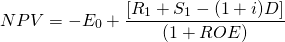
In the ROE approach, the analysis depends on how the asset is financed. In this approach, the cost of interest and debt payments is subtracted explicitly, and the initial investment is equal to the amount of equity invested, since the debt is paid directly to whoever supplies the investment. However, the debt D plus average interest costs charged at interest rate i (iD) are subtracted at the end of the period. The NPV for the ROE model is expressed as:
(8.19)
The fundamental rates of return identity. One of the issues to consider when comparing the ROE versus the ROA approach is that in equations (8.18) and (8.19), E0 and V0 are not equal because part of the acquisition of the investment is supported by debt, V0 = D0 + E0. The main point here is that the two approaches are not equivalent. We made this point when we derived Equation \ref{7.13} which is repeated here as Equation \ref{8.20}.
(8.20)
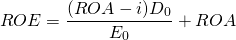
Notice that in Equation \ref{8.20}, if the cost of debt i is equal to the return on assets ROA, then ROA and ROE will be equal. But if i is less than the return on assets, then ROE > ROA. A homework problem at the end of this chapter asks you to explain this result. Equation (8.20) is so important in financial analysis that we give it a special name: the fundamental rates of return identity.
IRRs, ROAs, and ROEs
We earlier defined IRRs as the discount rate that corresponds to NPVs of zero. Now we illustrate how to find IRRs on assets and equity. The fundamental rates of return identity alerts us to the fact that IRRs calculated on equity invested in the project and assets invested in the project will not usually be equal. To find the IRRs on assets invested in the project, we charge the entire investment at the beginning of the period and include its liquidation value as a return at the end of the period. This approach ignores the fact that investments may be financed and paid for over the life of the investment and charging for the investment at the beginning of the project doesn’t accurately reflect its cash flow. This is the ROA approach. In this case, the ROA approach, we ignore financing because our interest is in the productive capacity of the long-term asset, independent of the terms under which it can be financed.
We illustrate how to find IRRs for assets (IRRA) in a simple example. Suppose the firm’s defender is a $1,000, non-depreciable investment that will earn $100 for one period and then will be liquidated at its acquisition price. We find the IRRA associated with $1,000 of assets invested in the defender by setting its NPV equal to zero in Equation \ref{8.18} and solving for ROA.
(8.21)
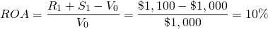
We find that the IRRA of the defender is equal to 10%.
Now reconsider the same example, except that the $500, or half of the defender, is financed at 9%. The other half of the investment, $500, is financed by the firm’s equity. We continue to assume that, after one period, the investment is liquidated for its acquisition value, the loan of $500 is repaid, and the firm recovers its investment of $500. The firm also earns in one period, $100, the same as before. But now it has to pay a rental fee for the use of the loan’s funds of 9% times $500, or $45. By setting the NPV model of the defender in Equation \ref{8.19} equal to zero, we can find its IRR associated with the firm’s equity (IRRE) in the project equal to.
(8.22)

Now the defender’s IRR on its equity is 11%. In this case, the firm gained access to the use of an asset because of financing. The gains from a lender providing the firm access to $500 of debt capital to acquire a $1000 investment using only $500 of its own money increased its earnings on its equity from 10% to 11%. Meanwhile the investment earned only 10%. The value of the financing increased the rate of return on equity by 1%.
ROE or ROA?
For a variety of reasons, financial managers may prefer to represent the defender’s IRR as the defender’s ROA or the defender’s ROE. However, this same manager must be careful to make sure that the cash flows associated with the challengers are consistent with the method used to find the IRR of the defender. If the IRR of the defender represents the defender’s ROE, then debt and interest costs should be accounted for explicitly. If the ROA of the defender is preferred, the cash flows associated with the challenger and the defender do not separate debt and interest costs from the calculations.
In practice, PV models appear to prefer the ROA approach, even though both approaches are valid and provide unique information. Nevertheless, the dominance of the ROA approach has resulted in the identification of ROAs as simply the IRR of the investment, a practice we will also adopt in the remainder of this book.
Summary and Conclusions
This chapter reviewed several different kinds of PV models. They differ because they are designed to answer different kinds of questions. Some PV models, NPV and IRR, help us rank alternative investments. Others like AE models can be used to find the optimal time for replacing an investment—or what our periodic loan payments will be. And still other PV models like the maximum bid (minimum sell) models help us know the maximum (minimum) we can offer to purchase (sell) an investment and still earn our defender’s IRR. Finally, still other PV models such as capitalization formulas and payback models offer at most a crude rule of thumb for evaluating and making investment decisions.
Regardless of the PV model type, they all have one measure in common: it is the opportunity cost of a defending investment represented by the discount rate. The discount rate is the ROA or the ROE of the defender that must be sacrificed to acquire the new or challenging investment. This construction of PV models emphasizes the important role of opportunity costs in the construction of PV models and reminds us that we focus on opportunity rather than direct costs when making applied economic decision.
Questions
- Explain the connection between investment questions and corresponding PV models.
- Suppose you found the maximum bid price for a purchase you are considering. What would you conclude from your calculations?
- Suppose that you found that an investment’s AE reached its maximum at year 10 while its NPV reached its maximum at 15 years. How would you interpret your results?
- When finding the ROE measure in Equation \ref{8.22}, we explicitly accounted for the debt used to finance the investment. However, when finding the ROA measure in Equation \ref{8.21}, we did not account for the debt used to finance the investment. Explain the difference between the two approaches.
- When comparing the ROAs and ROEs, we concluded that the ROE > ROA as long as the ROA was greater than the average interest rate on the debt used to finance an investment. Please explain these finding and provide an example on these results. Refer to the fundamental rates of return identity when formulating your answer.
- Provide numerical PV models in which you find an investment’s IRR and NPVs using ROA-IRR and ROE-IRR, AE, maximum bid price, and the investment’s payback period. Defend your choice of a discount rate.
- Explain how the “life of the investment” principle guarantees that all economic activity associated with an investment will be captured by its cash flow.
- Most of the time, we don’t identify discount rates in PV models as being either a ROE or a ROA. Instead we seem to prefer to identify the defender’s ROA with the letter “r”. Why do we tend to prefer ROA to ROE measures? Can you describe a case when it would be important to evaluate the projects using the defender’s ROE instead of its ROA?
- Assume you were considering one investment that could be financed from two different financial institutions. Thus the only difference between the projects were their cash flow associated with their use of debt capital. How would you proceed to rank the two investments?
- In a previous chapter, we calculated the rates of return on equity and rates of return on assets for HQN for the year 2018 for the entire firm. But this calculation was for only one year and included non-cash items in the calculation. What is different between IRRs calculated as ROA or ROE for the entire firm versus IRRs calculated as ROA or ROE in a PV model?
- Suppose you ranked two challengers using their IRRs and by finding their NPVs using the IRR of the defender. What would you conclude if the IRR and NPV ranking provided conflicting ranking?