The practicality of a strategy is the extent to which the strategy serves the purpose intended. Whereas facts are either true or false, practicality is a matter of degree. Tools for assessing practicality include SWOT, VRIO, breakeven analysis, projected financial statements, EPS-EBIT analysis, and matrices.
5.2.1: SWOT
The classic tool for assessing the practicality of a strategy is a list of considerations known as SWOT, standing for Strengths, Weaknesses, Opportunities, and Threats (Learned, Christiansen, Andrews, and Guth, 1969). Strengths and weaknesses are nominally factors internal to the organization, so the examination of an organization’s strengths and weaknesses is known as internal factor analysis. Opportunities and threats are nominally factors external to the organization, so the examination of these factors is known as external factor analysis. In fact, strengths do not exist without opportunities, and weaknesses do not exist without threats. An airline may employ many pilots who are excellent musicians, but musical talent is not the airline’s strength in the absence of an opportunity for the airline to apply its pilot-musicians to advance its business.
Accordingly, a listing of an organization’s strengths tends to overlap a listing of its opportunities. Likewise, a listing of its weaknesses tends to overlap a listing of its threats. To confound matters even more, a fact than one person considers a strength another may consider a weakness. If a firm has more employees than its competitor, for example, the firm has more resources at its disposal, apparently a strength. Yet, more employees also mean more difficulties in coordinating activities, apparently a weakness.
To address the overlap and varied interpretations, a four-part SWOT analysis can be reduced to a two-part ST analysis, that is, list only strengths and threats. Even better, reduce plurals to singulars, from strengths to strength, and threats to threat. The longer the list, the more the strongest item of each list becomes indistinct, reducing its value in strategy assessment. When only the best is good enough, the best strategy must be the one that builds on the firm’s primary strength and forestalls the firm’s most immediate threat.
5.2.2: VRIO
VRIO, standing for Value, Rare, costly to Imitate, and exploited by Organization (Barney, 2002), is a systematic means of identifying a firm’s core competencies that expands on strengths. The idea is to list the resources and capabilities of the firm that are valuable, which is to say that without them the firm would be less profitable or more vulnerable to threats. Then to cull the list to arrive at a shorter list of items that are rare, which is to say that few other firms have them. Then, to cull the second list to arrive at a final list of items that are costly for other firms to imitate. The items of the final list are the firm’s core competencies. Practical strategies are the ones that exploit core competencies. Strategies directed at unexploited core competencies are especially desirable.
In practice, each executive's VRIO listing is likely to differ from the list of every other executive, and attempts to reconcile the lists can be divisive. If some executive’s area of responsibility should be missing from the core-competency list, the implication on the standing of the executive whose area of responsibility is missing from the list is ominous.
5.2.3: Breakeven Analysis
The objective of breakeven analysis is to identify the point at which the firm’s net income will be zero. The firm will be marginally sustainable at this point, for in business, a positive net income is necessary for long-term survival. A strategy is less desirable to the extent it moves a profitable firm closer to its breakeven point.
Breakeven analysis is based on a model of a firm with a single product with cost of production falling into two categories: fixed and variable. For the model, whereas fixed costs do not change with production volume, variable cost rises linearly with production volume. Thus, Total Cost (C) equals Total Fixed Cost (F) plus Unit Variable Cost (v) multiplied by production volume (Q), as shown in Equation \ref{1}.
\[ C=F + vQ \label{1} \]
When unit price (p) is constant and the quantity produced is the quantity sold, total revenue (R) is the product of price and quantity, as shown in Equation \ref{2}.
\[R=pQ \label{2} \]
The breakeven quantity (Q*) is where C = R, as shown in Equation \ref{3}.
\[ pQ^{*} = F + v Q^{*} \label{3} \]
Applying algebra to Equation \ref{3}, the breakeven quantity is as shown in Equation \ref{4}.
\[ Q^{*} = \dfrac{F}{p - v} \label{4} \]
Thus, if Lucy’s lemonade stand is built with $20 worth of lumber, the fixed cost; if making lemonade requires $0.10 worth of lemons per cup, the variable cost; then if Lucy sells lemonade for $0.50 a cup, Lucy’s lemonade business will break even after she has sold $20 / ($0.50 - $0.10) = 50 cups of lemonade.
Although the particulars of Lucy’s lemonade stand may not apply to any sizeable everyday-world business, the basic principle is the same, but some adaptation usually is necessary. Many firms have more than one product and more than one model of each product. If sales of the products and models tend to rise and fall together, the firm’s breakeven can still be found even when an aggregated unit of output of the firm’s products and models is unavailable by applying Equation \ref{5}, derived by dividing both sides of Equation \ref{4} by current production volume (Q’).
\[ \dfrac{Q^{*}}{Q'} = \dfrac{F}{pQ' - vQ'} \label{5} \]
The left side of Equation \ref{5} is the breakeven point relative to current production volume. On the right side, pQ’ is current total revenue and vQ’ is current total variable cost. The figure for current total revenue appears on the firm’s current income statement. The figure for current total variable cost can be estimated from the same statement. If the firm’s policy is to adapt quickly to changes in sales by changing production-employment levels, then all of the firm’s current total cost of sales may be considered a reasonable estimate of current total variable cost. Otherwise, current total variable cost will be a fraction of current total cost of sales. The remaining current cost of sales, expenses, and interest charges sum to the firm’s current total fixed cost.
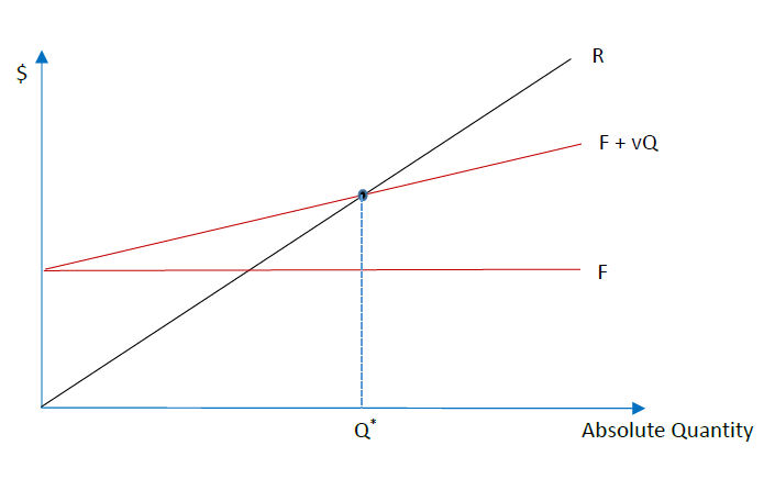
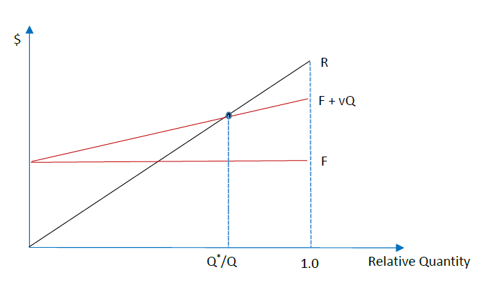
Graphing the relationships in the form of a breakeven chart, with quantity on the horizontal axis and the dollar amount on the vertical axis as illustrated in Figure \( \PageIndex{3} \) for Equation \ref{3}, and Figure \( \PageIndex{4} \), for Equation \ref{5}, can be helpful in a presentation. On both charts, the breakeven point is at the intersection between R, the total-revenue line, and F + vQ, the total-cost line. Breakeven charts can show the effect on profitability and the breakeven point of changing prices, marketing expenditures, and other contemplated actions.

Figure \( \PageIndex{3} \): Absolute-Quantity Breakeven Chart. Total Revenue (R), Total Fixed and Variable Costs (F + vQ), and Total Fixed Cost (F) vs. absolute quantity produced and sold. The crossing point is the breakeven quantity (Q*).

Figure \( \PageIndex{4} \): Relative-Quantity Breakeven Chart. Total Revenue (R), Total Fixed and Variable Costs (F + vQ), and Total Fixed Cost (F) vs. relative quantity produced and sold. The crossing point is the breakeven quantity relative to current quantity produced and sold (Q* / Q).
5.2.4: Projected Financial Statement
Projected, also known as pro forma, financial statements are especially useful for assessing the practicality of a strategy that includes several elements that must be coordinated. Launching a new product epitomizes a strategy of this kind. Expenses must be incurred to finalize development of the product, followed by manufacturing, advertising, and delivery of the product to customers. Financing through borrowing or sales of shares might be necessary. In general, projecting the financial statements is necessary to ascertain how much financing is needed and when it is needed.
A complete set of project financial statements includes three scenarios: pessimistic, optimistic, and likely. To proceed, begin with the likely scenario. Project first the items of the income statement, followed by those of the balance sheet.
On a spreadsheet, assign a column to each year, starting with the first year of the strategy and ending with the third year after the product reaches its market. Starting with revenue, enter on the spreadsheet the likely annual revenue of the strategy for each of the five years. Follow by projecting the cost of the goods or services over the same periods, and then the expenses from the most recent year to the last year projected. You can simplify your work on some items by entering formulas rather than numbers. For example, enter cost of goods or services as a ratio of revenue, gross margin as revenue minus cost of goods or services, and so forth.
Enter zeros for interest expenses beyond those of existing debt. You will return to interest expense later, if after completing the projections you find that borrowing is needed. When you reach net income after taxes, enter dividends or withdrawals, as the case may be, following existing policy on the payment. The item following dividends or withdrawals will be the contribution to retained earnings. Add this amount to the firm’s retained earnings of the previous year to arrive at the retained earnings of the income-statement-ending year.
After projecting retained earnings over all the years of the projected income statement, project the remaining items of the balance sheet, excepting cash. Account receivables may be reasonably projected as a fraction of revenue. Likewise, inventory and accounts payable may be reasonably projected as fractions of cost of goods or services. Use a summative formula to compute Total Liabilities and Equity. Use a reference formula to assure that the figure for Total Assets is the same as the one for Total Liabilities and Equity. Use a subtractive formula to compute Cash. Thus, Cash is the plug account that assure that the balance sheet balances, so that Total Assets = Total Liabilities and Equity, as it must.
Examine the cash account. If it is low or negative, enter the combination of long-term debt and capital sufficient for positive cash, reasonable current and quick ratios, and acceptable long-term debt to equity ratios. A model for choosing between debt and equity financing is discussed in Part 5.2.5.
To finalize the projection, replace the zero-interest-expense items of the projected income statement with formulas that compute interest expense as a percentage of long-term and other debt that may be in the projected balance sheet. Tweak dividends or withdrawals, long-term debt, and capital until the liquidity ratios are about right for every year projected.
Having projected the likely scenario, proceed to projecting the pessimistic and optimistic scenarios, using the spreadsheet of the likely scenario as the template. For presentations, apply the graphic features of the spreadsheet to show charts of revenue, net income after taxes, long-term debt, and other items that might be of interest.
5.2.5: EPS-EBIT Analysis
The viability of a strategy must be assured before its financing is addressed, for a wager that is not a good bet is not a good bet irrespective of who fronts the money for the bet. Viability assured, the analysis of earnings per share (EPS) relative to earnings before interest and taxes (EBIT) addresses the question of whether the financing of a corporation’s strategy should be by debt or equity. Two examples highlight the issue.
Bob has a safe investment that will surely earn more than the interest that Bob must pay to borrow the needed money from his bank. The investment might be to buy materials for renovating a house for which Bob has a signed contract from the homeowner. Should Bob ask his bank for a loan, or ask an investor he knows to invest in the project for a share of the outcome, a likely profit and an unlikely investment loss?
Sue has a risky investment that will lose money if she fails, but win her a lucrative prize if she succeeds. The investment might be to employ an assistant to help her develop artificial-intelligence software for a national competition. Should Sue ask her bank for a loan, or ask an investor she knows to invest in the competition for a share of the outcome, an unlikely profit and a likely investment loss?
The answer might seem obvious. Bob should ask his bank (debt financing), and Sue should ask her investor (equity financing). In principle, whereas debt financing is more practical when the risk is low, equity financing is more practical when the risk is high. Between the extremes, the answer will depend on the interest rate of the debt relative to the share of the project that must be given up for the equity, moderated by tax, legal, and personal concerns. These considerations can be clarified with algebra and a graph.
Consider an EPS-maximizing linear model (David & David, 2017) whereby debt to finance strategic investments incurs an interest payment (I). Consider also that a constant corporate income tax rate (r) applies to earnings net of all interest payments, so that the firm’s projected income-tax payment is (EBIT – I)r and its projected after-tax earnings is therefore (EBIT – I) – (EBIT – I)r. EPS is the firm’s after-tax earnings divided by its number of shares outstanding (n). Accordingly, if the firm’s strategy should be financed with debt only, then its projected EPS is derived by applying Equation \ref{6}.
\[ \text{EPS} = \dfrac{\left ( \text{EBIT}-I \right ) - \left ( \text{EBIT}-I \right ) \left ( 1-r \right ) }{n} = \dfrac{\left ( \text{EBIT}-I \right )\left ( 1-r \right )}{n} \label{6} \]
On the other hand, if the strategy is financed with equity only, a number of new shares (m) will have to be issued in lieu of debt, but with no debt, no interest payment will have to be made, so I = 0. In this case, the firm’s projected EPS is derived by applying Equation \ref{7}.
\[ \text{EPS} = \dfrac{\text{EBIT} \left ( 1-r \right )}{n+m} \label{7} \]
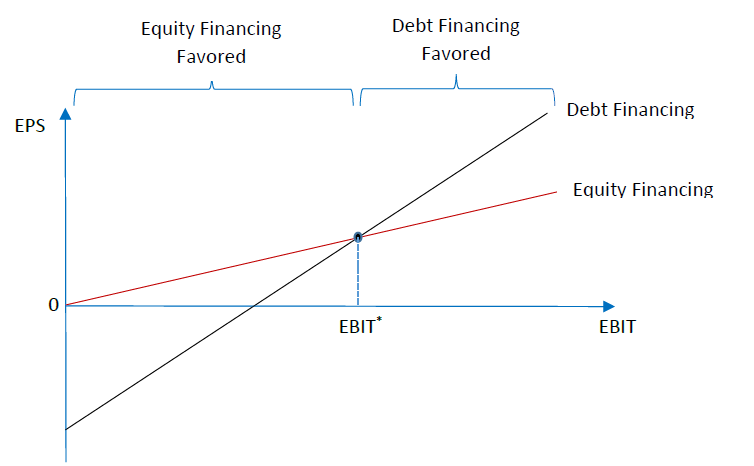
Thus, for the general case of necessary payments of interest on debt (I > 0) and of reasonable taxes on corporate income (1 > r > 0), when EBIT = 0, EPS for debt-only financing (Equation \ref{6} must be negative and EPS for equity-only financing must be zero (Equation \ref{7}). These two points are shown in Figure \( \PageIndex{3} \), a graph of EPS relative to EBIT.

Figure \( \PageIndex{3} \): EPS-EBIT Chart.
For both debt-only and equity-only financing, EPS rises linearly with EBIT, but the slope of the curve (actually a straight line) is greater for debt-only financing. To see this, Equation \ref{8} rearranges Equation \ref{6} in slope-intercept form to show that the slope of the curve for debt-only financing, (1 – r) / n, differs only from the slope for equity-only financing (Equation \ref{7}), (1 – r) / (n + m), in that the equity-only denominator is greater by m. Since equity financing implies that m > 0, the equity-only slope must be smaller.
\[ \text{EPS} = \dfrac{\text{EBIT} \left ( 1-r \right )}{n} - \dfrac{I \left ( 1-r \right )}{n} \label{8} \]
The critical point is at the intersection of the two curves. Debt-only financing is favored for EBIT above this point, whereas equity-only financing is favored below it.
Algebraically, the critical point (EBIT*) is when the equity-only EPS (Equation \ref{7}) equals the debt-only EPS (Equation \ref{8}). At that point, Equation \ref{9} holds. Isolating EBIT* on the left gives rise to Equation \ref{10}.
\[ \text{EPS} = \dfrac{\text{EBIT}^{*} \left ( 1-r \right )}{n+m} = \dfrac{\text{EBIT}^{*} \left ( 1-r \right )}{n} - \dfrac{I \left ( 1-r \right )}{n} \label{9} \]
\[ \text{EBIT}^{*} = I\left ( \dfrac{n}{m} +1 \right ) \label{10} \]
Confirming intuition, Equation \ref{10} shows that debt financing is preferred over equity financing (EBIT* is smaller) when the interest payment (I) is lower and more shares must be issued relative to those outstanding (n/m is smaller). Math sharpens intuition.
5.2.6: Matrices
Matrices, useful for showing the practicality of a strategy along two or more dimensions, add precision to qualitative arguments. That the axes and associated numbers of a matrix are usually imprecise is limitation of data, rather than a fault in the technique itself.
5.2.6.1: Product positioning matrix
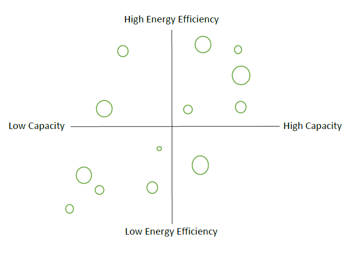
Matrices are especially useful in marketing, by breaking down the often-ambiguous idea of product desirability into more tangible attributes. A washing machine, for example, can have two attributes: capacity and energy efficiency. A matrix of available washing machines in a market can show the relative placement of a proposed new machine among those already available. A matrix of this kind is a product-positioning matrix, also known as a perceptual map, as illustrated in Figure \( \PageIndex{4} \). On the figure, each washing-machine model is represented by a circle whose size corresponds to its share of the market. The practicality of a new model is assessed by visually observing its place on the matrix. Generally, a new model should be positioned high on the attribute that customers uniformly desire (e.g., energy efficiency) and away from other models on the attribute that vary in desirability among customers (e.g., capacity).

Figure \( \PageIndex{4} \): Product Positioning Matrix of Washing Machines.
To arrive at a single comprehensive score for products with several uniformly desirable attributes, assign each attribute a weight corresponding to its judged importance to the market (e.g., .40 for energy efficiency, .25 for water efficiency, and .35. for noise). Then ask a panel representative of the customers to score the attributes of each model on a fixed rating scale, say from 1 to 5. For each model, multiple the panel’s average scores across the attributes (e.g., 4 for energy efficiency, 5 for water efficiency, and 2 for noise) by their weights and sum the weighted scores across all attributes to arrive at a single comprehensive score of the product’s rated desirability for that market (e.g., 4 × .4 + 5 × .25 + 2 × .35 = 3.55). If the weights are set such that they sum to one (.40 + .25 + .35 = 1.0), then the comprehensive score will fall conveniently within the range of the rating scale (e.g., 1 to 5).
5.2.6.2: Product portfolio matrix
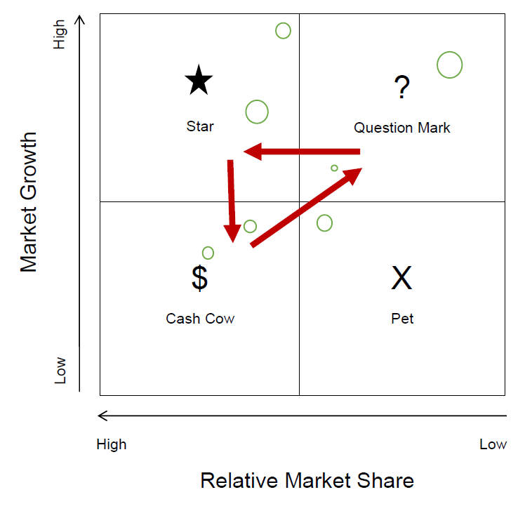
A conglomerate doing business in several markets may have market shares and market growth that differ by market. In this case, a market-share, market-growth matrix can highlight the practicality of a strategy that is more or less aggressive, a point made by Henderson (1970) of the Boston Consulting Group (BCG), whose product portfolio matrix is well known. Unlike the product-positioning matrix, which shows competing models of a single market, the product portfolio matrix shows non-competing businesses in different markets.
The BCG product portfolio matrix is unusual in two respects. First, instead of absolute market shares, the matrix uses relative market share, computed by dividing the absolute market share of the business by the market share of the competitor with the highest market share. Thus, if the absolute market shares of the three competitors are 30%, 25%, and 15%, then the relative market shares of those competitors are 30% / 25% = 1.2, 25% / 30% = 0.83, and 15% / 30% = 0.50, respectively. Second, the matrix shows relative market share as falling, rather than rising, with distance from the origin. An example of a product portfolio matrix is shown in Figure \( \PageIndex{5} \).

Figure \( \PageIndex{5} \): Product Portfolio Matrix.
In Figure \( \PageIndex{5} \), businesses appear as circles, the size of which corresponds to each business’s percentage of the firm’s total revenue. Henderson suggests that a strategy of investment is practical for question marks, businesses with low relative market share in an industry with high market growth. The investment objective is to turn question marks to stars, businesses with high relative market share in an industry with high market growth. To keep up with market growth, stars require continued investment, so they generally generate little cash. Eventually, however, market growth must diminish, in which case the stars become cash cows, businesses with high relative market share in a market with low growth. A strategy of maintenance is appropriate for cash cows, for their profitability would not rise with further investments. The cash they generate should be reinvested in question marks, completing the cycle of cash cows → question marks → stars → cash cows.
A disinvestment strategy is practical for pets, originally called dogs. These are businesses with low relative market share in a market with little to no market growth. Relative to the other businesses of the firm, they are failures.
The line dividing high and low relative market shares depends on how the markets of the various businesses are defined. The narrower the definition, the fewer the number of competing firms and therefore the higher the market share of each firm. The ambiguity makes the product portfolio matrix more of an illustrative technique than a theory of investment. One could start with 1.0 as the dividing line. If none of the firm’s businesses appears to the left of the line, which occurs when none has the highest absolute share of its market, then set the line to 0.5 or lower.
The line dividing high and low market growth depends on how the economy is defined. The definition of the economy should include all the areas in which the firm does business. The line of division could be set at 0% or at the long-term growth rate of the defined economy, which is about 5% a year globally, about 2% a year for the United States, and more or less elsewhere.
5.2.6.3: Porter’s generic strategies
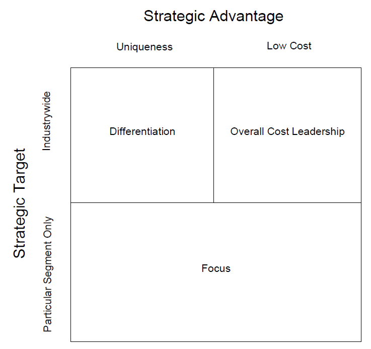
Porter’s (1980) argument for the practicality of three so-called generic strategies and the impracticality of one is based on a matrix of strategic target vs. strategic advantage, as illustrated in Figure \( \PageIndex{6} \). Strategic target refers to the population that the firm’s product is intended to serve, and strategic advantage refers to the extent to which the product is, in the customer’s perception, either superior (uniqueness) or inexpensive (low cost), the presumption being that firms maximize profit, so a firm with a superior product would not sell the product for a low price.

Figure \( \PageIndex{6} \): Porter's Generic Strategies.
Porter argues that if a firm can keep cost below that of its competitors, an overall cost leadership strategy of pricing the product low to attract an industrywide market is practical. Also practical is a differentiation strategy of making the product appear superior in the eyes of the customer, either because of branding or desirable features or both, so that the product remains attractive industrywide even when priced higher than the prices of its competitors. Also practical is a focus strategy of reaching just a segment of the industry with an inexpensive product, cost focus; or a higher-priced unique product, differentiation focus. Porter disparages any strategy that is not among the three as stuck in the middle.


