3.22: Finding Equilibrium

Learning Objectives

• Explain what happens to supply, demand, and equilibrium when there is a change in both supply and demand

You have seen how changes in weather can influence supply and changes in consumer preferences can reduce demand, but what happens when both supply and demand are changing? Often changes in an economy affect both the supply and the demand curves, making it more difficult to assess the impact on the equilibrium price. Let’s review one such example.

Figure 1.Money and Mail. How do changes at the post office impact other aspects of the economy?

First, consider the following questions:

1. Suppose postal workers are successful in obtaining a pay raise from the U.S. Postal Service. Will this affect the supply or the demand for first-class mail? Why? Which determinant of demand or supply is being affected? Show graphically with before and after curves on the same axes. How will this change the equilibrium price and quantity of first-class mail?
2. How do you imagine the invention of email and text messaging affected the market for first-class mail? Why? Which determinant of demand or supply is being affected? Show graphically with before and after curves on the same axes. How will this change the equilibrium price and quantity of first-class mail?
3. Suppose that postal workers get a pay raise and email and text messaging become common. What will the combined impact be on the equilibrium price and quantity of first-class mail?

In order to complete a complex analysis like this it’s helpful to tackle the parts separately and then combine them, while thinking about possible interactions between the two parts that might affect the overall outcome. Let’s use the four-step process.

Exercise: Postal Service

Part 1: A Pay Raise for Postal Workers

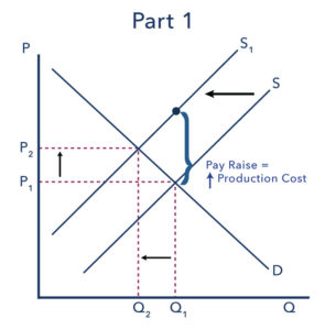
Step 1. Draw a demand and supply model to illustrate what the market for the U.S. Postal Service looks like before this scenario starts. The demand curve D and the supply curve S show the original relationships.

Figure 2. The supply and demand curves for the U.S. Postal Service after a pay raise for postal workers.

Step 2. Will a pay raise for postal workers affect supply or demand?

[reveal-answer q=”337241″]Show Answer[/reveal-answer]
[hidden-answer a=”337241″]Labor compensation is a cost of production. A change in production costs cause a change in supply for the Postal Service.[/hidden-answer]

Step 3. Is the effect on supply positive or negative?

[reveal-answer q=”654161″]Show Answer[/reveal-answer]
[hidden-answer a=”654161″]Higher labor compensation leads to a lower quantity supplied of postal services at every given price, causing the supply curve for postal services to shift to the left, from S to S₁.[/hidden-answer]

Step 4. Compare the new equilibrium price and quantity to the original equilibrium price.

[reveal-answer q=”20641″]Show Answer[/reveal-answer]
[hidden-answer a=”20641″]The new equilibrium occurs at a lower quantity and a higher price than the original equilibrium.[/hidden-answer]

A pay raise for postal workers would represent an increase in the cost of production for the Postal Service. Production costs are a factor that influences supply; thus, the pay raise should decrease the supply of first-class mail, shifting the supply curve vertically by the amount of the pay raise. Intuitively, all else held constant, the Postal Service would like to charge a higher price that incorporates the higher cost of production. That is not to say the higher price will stick. From the graph (Figure 1), it should be clear that at that higher price, the quantity supplied is greater than the quantity demanded—thus there would be a surplus, indicating that the price the Postal Service desires is not an equilibrium price. Or to put it differently, at the original price (P₁), the decrease in supply causes a shortage driving up the price to a new equilibrium level (P₂). Note that the price doesn’t rise by the full amount of the pay increase. In short, a leftward shift in the supply curve causes a movement up the demand curve, resulting in a lower equilibrium quantity (Q₂) and a higher equilibrium price (P₂).

Part 2: The Effect of Email and Text Messaging

Step 1. We’ve already seen how a pay raise will shift the supply curve to the left. Now let’s consider how the invention of email and text messaging affects the market for first-class mail. Begin by drawing a demand and supply model reflecting this relationship.

Figure 3. The impact of email and text messages on the snail mail market.

Step 2. Does email and text messaging affect supply or demand?

[reveal-answer q=”655707″]Show Answer[/reveal-answer]
[hidden-answer a=”655707″]A change in tastes away from snail mail toward digital messages will cause a change in demand for the Postal Service.[/hidden-answer]

Step 3. Is the effect on demand positive or negative?

[reveal-answer q=”193138″]Show Answer[/reveal-answer]
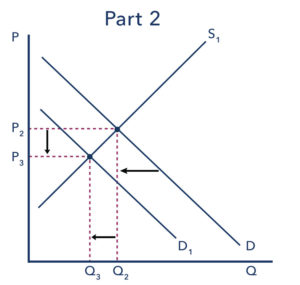
[hidden-answer a=”193138″]A change in tastes away from snail mail toward digital messages causes lower quantity demanded of postal services at every given price, causing the demand curve for postal services to shift to the left, from D to D₁.[/hidden-answer]

Step 4. Compare the new equilibrium price and quantity to the original equilibrium price.

[reveal-answer q=”473433″]Show Answer[/reveal-answer]
[hidden-answer a=”473433″]The new equilibrium occurs at a lower quantity and a lower price than the original equilibrium.[/hidden-answer]

To summarize, since many people find email and texting more convenient than sending a letter, we can assume that tastes and preferences for first-class mail will decline. This decrease in demand is shown by a leftward shift in the demand curve and a movement along the supply curve, which creates a surplus in first-class mail at the original price (shown as P₂). The shortage causes a decrease in the equilibrium price (to P₃) and a decrease in the equilibrium quantity (to Q₃). Intuitively, less demand for first-class mail leads to a lower equilibrium quantity and (ceteris paribus) a lower equilibrium price.

Part 3: Combining Factors

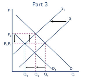
Parts 1 and 2 are straightforward, but when we put them together it becomes more complex. Think about it this way: in Part 1, the equilibrium quantity fell due to decreased supply. In Part 2, the equilibrium quantity also fell, this time due to the decreased demand. So putting the two parts together, we would expect to see the final equilibrium quantity (Q₃) to be smaller than the original equilibrium quantity (Q₁). So far, so good.

Now consider what happens to the price. In Part 1, the equilibrium price increased due to the reduction in supply. But in Part 2, the equilibrium price decreased due to the decrease in demand! What will happen to the equilibrium price? The net effect on price can’t be determined without knowing which curve shifts more, demand or supply. The equilibrium price could increase, decrease, or stay the same. You just can’t tell from graphical analysis alone. This is not unusual. When both curves shift, typically we can determine the overall effect on price or on quantity, but not on both. In this case, we determined the overall effect on the equilibrium quantity, but not on the equilibrium price.

Figure 4. Decreased supply and decreased demand cause the equilibrium quantity to fall (Q3 is be smaller than the original equilibrium quantity of Q1). It is hard to pinpoint what happens to the price, however, as it may decline with the shrinking demand, but also increase with production costs.

Try It

https://assessments.lumenlearning.co...sessments/7452

https://assessments.lumenlearning.co...sessments/7453

 

Contributors and Attributions

CC licensed content, Original

• Worked Example: Supply and Demand. Authored by: Steven Greenlaw and Lumen Learning. License: CC BY: Attribution
• Modification, adaptation, and original content.. Provided by: Lumen Learning. License: CC BY: Attribution

CC licensed content, Shared previously

• Mail truck. Authored by: ArtisticOperations. Provided by: Pixabay. Located at: https://pixabay.com/en/mail-truck-mail-clerk-mailman-3248139/. License: CC0: No Rights Reserved