Business LibreTexts

1.12: Creating and Interpreting Graphs

  • Page ID
    47261
  • \( \newcommand{\vecs}[1]{\overset { \scriptstyle \rightharpoonup} {\mathbf{#1}} } \)

    \( \newcommand{\vecd}[1]{\overset{-\!-\!\rightharpoonup}{\vphantom{a}\smash {#1}}} \)

    \( \newcommand{\id}{\mathrm{id}}\) \( \newcommand{\Span}{\mathrm{span}}\)

    ( \newcommand{\kernel}{\mathrm{null}\,}\) \( \newcommand{\range}{\mathrm{range}\,}\)

    \( \newcommand{\RealPart}{\mathrm{Re}}\) \( \newcommand{\ImaginaryPart}{\mathrm{Im}}\)

    \( \newcommand{\Argument}{\mathrm{Arg}}\) \( \newcommand{\norm}[1]{\| #1 \|}\)

    \( \newcommand{\inner}[2]{\langle #1, #2 \rangle}\)

    \( \newcommand{\Span}{\mathrm{span}}\)

    \( \newcommand{\id}{\mathrm{id}}\)

    \( \newcommand{\Span}{\mathrm{span}}\)

    \( \newcommand{\kernel}{\mathrm{null}\,}\)

    \( \newcommand{\range}{\mathrm{range}\,}\)

    \( \newcommand{\RealPart}{\mathrm{Re}}\)

    \( \newcommand{\ImaginaryPart}{\mathrm{Im}}\)

    \( \newcommand{\Argument}{\mathrm{Arg}}\)

    \( \newcommand{\norm}[1]{\| #1 \|}\)

    \( \newcommand{\inner}[2]{\langle #1, #2 \rangle}\)

    \( \newcommand{\Span}{\mathrm{span}}\) \( \newcommand{\AA}{\unicode[.8,0]{x212B}}\)

    \( \newcommand{\vectorA}[1]{\vec{#1}}      % arrow\)

    \( \newcommand{\vectorAt}[1]{\vec{\text{#1}}}      % arrow\)

    \( \newcommand{\vectorB}[1]{\overset { \scriptstyle \rightharpoonup} {\mathbf{#1}} } \)

    \( \newcommand{\vectorC}[1]{\textbf{#1}} \)

    \( \newcommand{\vectorD}[1]{\overrightarrow{#1}} \)

    \( \newcommand{\vectorDt}[1]{\overrightarrow{\text{#1}}} \)

    \( \newcommand{\vectE}[1]{\overset{-\!-\!\rightharpoonup}{\vphantom{a}\smash{\mathbf {#1}}}} \)

    \( \newcommand{\vecs}[1]{\overset { \scriptstyle \rightharpoonup} {\mathbf{#1}} } \)

    \( \newcommand{\vecd}[1]{\overset{-\!-\!\rightharpoonup}{\vphantom{a}\smash {#1}}} \)

    \(\newcommand{\avec}{\mathbf a}\) \(\newcommand{\bvec}{\mathbf b}\) \(\newcommand{\cvec}{\mathbf c}\) \(\newcommand{\dvec}{\mathbf d}\) \(\newcommand{\dtil}{\widetilde{\mathbf d}}\) \(\newcommand{\evec}{\mathbf e}\) \(\newcommand{\fvec}{\mathbf f}\) \(\newcommand{\nvec}{\mathbf n}\) \(\newcommand{\pvec}{\mathbf p}\) \(\newcommand{\qvec}{\mathbf q}\) \(\newcommand{\svec}{\mathbf s}\) \(\newcommand{\tvec}{\mathbf t}\) \(\newcommand{\uvec}{\mathbf u}\) \(\newcommand{\vvec}{\mathbf v}\) \(\newcommand{\wvec}{\mathbf w}\) \(\newcommand{\xvec}{\mathbf x}\) \(\newcommand{\yvec}{\mathbf y}\) \(\newcommand{\zvec}{\mathbf z}\) \(\newcommand{\rvec}{\mathbf r}\) \(\newcommand{\mvec}{\mathbf m}\) \(\newcommand{\zerovec}{\mathbf 0}\) \(\newcommand{\onevec}{\mathbf 1}\) \(\newcommand{\real}{\mathbb R}\) \(\newcommand{\twovec}[2]{\left[\begin{array}{r}#1 \\ #2 \end{array}\right]}\) \(\newcommand{\ctwovec}[2]{\left[\begin{array}{c}#1 \\ #2 \end{array}\right]}\) \(\newcommand{\threevec}[3]{\left[\begin{array}{r}#1 \\ #2 \\ #3 \end{array}\right]}\) \(\newcommand{\cthreevec}[3]{\left[\begin{array}{c}#1 \\ #2 \\ #3 \end{array}\right]}\) \(\newcommand{\fourvec}[4]{\left[\begin{array}{r}#1 \\ #2 \\ #3 \\ #4 \end{array}\right]}\) \(\newcommand{\cfourvec}[4]{\left[\begin{array}{c}#1 \\ #2 \\ #3 \\ #4 \end{array}\right]}\) \(\newcommand{\fivevec}[5]{\left[\begin{array}{r}#1 \\ #2 \\ #3 \\ #4 \\ #5 \\ \end{array}\right]}\) \(\newcommand{\cfivevec}[5]{\left[\begin{array}{c}#1 \\ #2 \\ #3 \\ #4 \\ #5 \\ \end{array}\right]}\) \(\newcommand{\mattwo}[4]{\left[\begin{array}{rr}#1 \amp #2 \\ #3 \amp #4 \\ \end{array}\right]}\) \(\newcommand{\laspan}[1]{\text{Span}\{#1\}}\) \(\newcommand{\bcal}{\cal B}\) \(\newcommand{\ccal}{\cal C}\) \(\newcommand{\scal}{\cal S}\) \(\newcommand{\wcal}{\cal W}\) \(\newcommand{\ecal}{\cal E}\) \(\newcommand{\coords}[2]{\left\{#1\right\}_{#2}}\) \(\newcommand{\gray}[1]{\color{gray}{#1}}\) \(\newcommand{\lgray}[1]{\color{lightgray}{#1}}\) \(\newcommand{\rank}{\operatorname{rank}}\) \(\newcommand{\row}{\text{Row}}\) \(\newcommand{\col}{\text{Col}}\) \(\renewcommand{\row}{\text{Row}}\) \(\newcommand{\nul}{\text{Nul}}\) \(\newcommand{\var}{\text{Var}}\) \(\newcommand{\corr}{\text{corr}}\) \(\newcommand{\len}[1]{\left|#1\right|}\) \(\newcommand{\bbar}{\overline{\bvec}}\) \(\newcommand{\bhat}{\widehat{\bvec}}\) \(\newcommand{\bperp}{\bvec^\perp}\) \(\newcommand{\xhat}{\widehat{\xvec}}\) \(\newcommand{\vhat}{\widehat{\vvec}}\) \(\newcommand{\uhat}{\widehat{\uvec}}\) \(\newcommand{\what}{\widehat{\wvec}}\) \(\newcommand{\Sighat}{\widehat{\Sigma}}\) \(\newcommand{\lt}{<}\) \(\newcommand{\gt}{>}\) \(\newcommand{\amp}{&}\) \(\definecolor{fillinmathshade}{gray}{0.9}\)

    Learning Objectives

    • Explain how to construct a simple graph that shows the relationship between two variables

    It’s important to know the terminology of graphs in order to understand and manipulate them. Let’s begin with a visual representation of the terms (shown in Figure 1), and then we can discuss each one in greater detail.
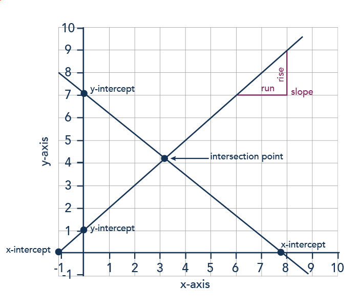
    A standard graph with an x- and y-axis. There is a positive slope line and a negative slope line. Where the lines cross the x-axis is a x-intercept. Where the lines cross the y-axis is a y-intercept. Where the two lines cross is the intercept. Slope is defined as rise over run, or the slant of the line.
    Figure 1. Graph Terminology.

    Throughout this course we will refer to the horizontal line at the base of the graph as the x-axis. We will refer to the vertical line on the left hand side of the graph as the y-axis. This is the standard convention for graphs. In economics, we commonly use graphs with price (p) represented on the y-axis, and quantity (q) represented on the x-axis.

    An intercept is where a line on a graph crosses (“intercepts”) the x-axis or the y-axis. Mathematically, the x-intercept is the value of x when y = 0. Similarly, the y-intercept is the value of y when x = 0. You can see the x-intercepts and y-intercepts on the graph above.

    The point where two lines on a graph cross is called an intersection point.

    The other important term to know is slope. The slope tells us how steep a line on a graph is as we move from one point on the line to another point on the line. Technically, slope is the change in the vertical axis divided by the change in the horizontal axis. The formula for calculating the slope is often referred to as the “rise over the run”—again, the change in the distance on the y-axis (rise) divided by the change in the x-axis (run).

    Now that you know the “parts” of a graph, let’s turn to the equation for a line:

    y = mx + b

    In any equation for a line, m is the slope and b is the y-intercept.

    Let’s use the same equation we used earlier, in the section on solving algebraic equations, y = 9 + 3x, which can also be written as:

    y = 3x + 9

    In this equation for a line, the b term is 9 and the m term is 3. The table below shows the values of x and y for this equation. To construct the table, just plug in a series of different values for x, and then calculate the resulting values for y.

    Values for the Slope Intercept Equation
    x y
    0 9
    1 12
    2 15
    3 18
    4 21
    5 24
    6 27
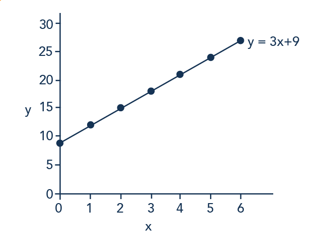
    Next we can place each of these points on a graph. We can start with 0 on the x-axis and plot a point at 9 on the y-axis. We can do the same with the other pairs of values and draw a line through all the points, as on the graph in Figure 2, below.
    The line graph shows the following approximate points: (0, 9); (1, 12); (2, 15); (3, 18); (4, 21); (5, 24); (6, 27).
    Figure 2. Slope and Algebra of a Straight Line.

    This example illustrates how the b and m terms in an equation for a straight line determine the position of the line on a graph. As noted above, the b term is the y-intercept. The reason is that if x = 0, the b term will reveal where the line intercepts, or crosses, the y-axis. In this example, the line hits the vertical axis at 9. The m term in the equation for the line is the slope. Remember that slope is defined as rise over run; the slope of a line from one point to another is the change in the vertical axis divided by the change in the horizontal axis. In this example, each time the x term increases by 1 (the run), the y term rises by 3. Thus, the slope of this line is therefore 3/1 = 3. Specifying a y-intercept and a slope—that is, specifying b and m in the equation for a line—will identify a specific line. Although it is rare for real-world data points to arrange themselves as a perfectly straight line, it often turns out that a straight line can offer a reasonable approximation of actual data.

    Watch It

    Watch this video to take a closer look at graphs and how variables can be represented in graph form. NOTE: Around the two-minute mark, the narrator inadvertently says “indirect,” rather than “inverse.” This is corrected later in the video.

    An interactive or media element has been excluded from this version of the text. You can view it online here: http://pb.libretexts.org/mlum/?p=70

    Glossary

    [glossary-page][glossary-term]intercept: [/glossary-term]
    [glossary-definition]the point on a graph where a line crosses the vertical axis or horizontal axis [/glossary-definition][glossary-term]slope: [/glossary-term][glossary-definition]the change in the vertical axis divided by the change in the horizontal axis [/glossary-definition][glossary-term]variable: [/glossary-term][glossary-definition]a quantity that can assume a range of values [/glossary-definition][glossary-term]x-axis: [/glossary-term][glossary-definition]the horizontal line on a graph, commonly represents quantity (q) on graphs in economics [/glossary-definition][glossary-term]y-axis: [/glossary-term][glossary-definition]the vertical line on a graph, commonly represents price (p) on graphs in economics [/glossary-definition][/glossary-page]

    CC licensed content, Original
    CC licensed content, Shared previously

    1.12: Creating and Interpreting Graphs is shared under a not declared license and was authored, remixed, and/or curated by LibreTexts.

    • Was this article helpful?