26.2: New Keynesians
- Page ID
- 32305
- How does the new Keynesian model differ from the new classical macroeconomic model?
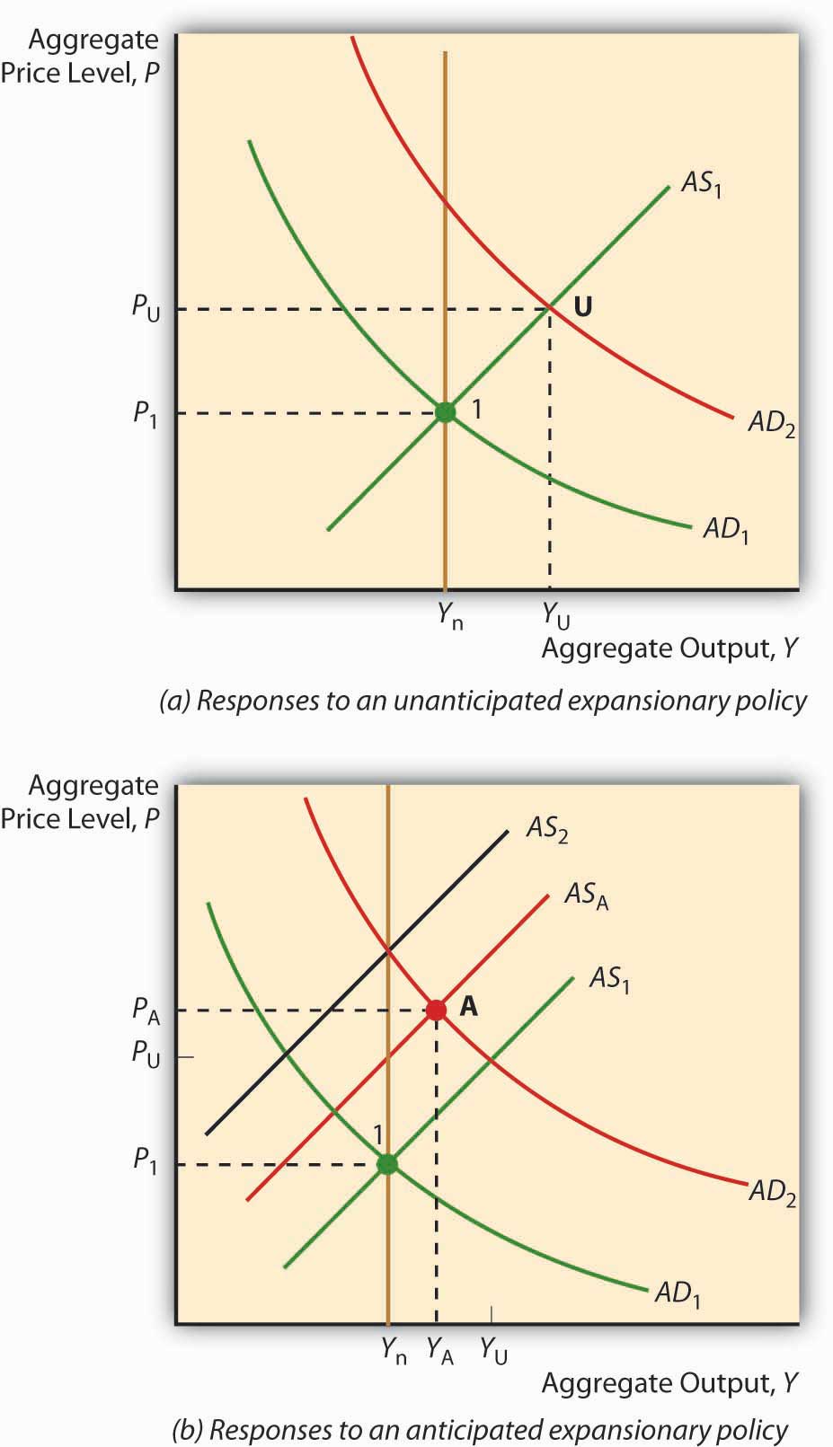
The new classical macroeconomic model aids the cause of nonactivists, economists who believe that policymakers should have as little discretion as possible, because it suggests that policymakers are more likely to make things (especially P* and Y*) worse rather than better. The activists could not stand idly by but neither could they ignore the implications of Lucas’s critique of prerational expectations macroeconomic theories. The result was renewed research that led to the development of what is often called the new Keynesian model. That model directly refutes the notion that wages and prices respond immediately and fully to expected changes in P*. Workers in the first year of a three-year labor contract, for example, can’t push their wages higher no matter their expectations. Firms are also reluctant to lower wages even when unemployment is high because doing so may exacerbate the principal-agent problem in the form of labor strife, everything from slacking to theft, to strikes. New hires might be brought in at lower wages, but if turnover is low, that process could take years to play out. Similarly, companies often sign multiyear fixed-price contracts with their suppliers and/or distributors, effectively preventing them from acting on new expectations of P*. In short, wages and prices are “sticky” and hence adjustments are slow, not instantaneous as assumed by Lucas and company.
If that is the case, as Figure 26.2 shows, anticipated policy can and does affect Y*, although not as much as an unanticipated policy move of the same type, timing, and magnitude would. The Takeaway is that an EMP, even if it is anticipated, can have positive economic effects (Y* > Ynrl for some period of time), but it is better if the central bank initiates unanticipated policies. And there is still a chance that policies will backfire if wages and prices are not as sticky as people believe, or if expectations and actual policy implementation differ greatly.

Adherents of the new classical macroeconomic model believe that stabilization policy, the attempt to keep output fluctuations to a minimum, is likely to aggravate changes in Y* as policymakers and economic agents attempt to outguess each other—policymakers by initiating unanticipated policies and economic agents by anticipating them! New Keynesians, by contrast, believe that some stabilization is possible because even anticipated policies have some short-run effects due to wage and price stickiness.
Stop and Think Box
In the early 1980s, U.S. President Ronald Reagan and U.K. Prime Minister Margaret Thatcher announced the same set of policies: tax cuts, more defense spending, and anti-inflationary monetary policy. In both countries, sharp recessions with high unemployment occurred, but the inflation beast was eventually slain. Why did that particular outcome occur?
Tax cuts plus increased defense spending meant larger budget deficits, which spells EFP and a rightward shift in AD. That, of course, ran directly counter to claims about fighting inflation, which were not credible and hence not anticipated. But the Fed and the Bank of England did get tough by raising overnight interest rates to very high levels (about 20 percent!). As a result, the happy conclusions of the new classical macroeconomic model did not hold. The AS curve shifted hard left, while the AD curve did not shift as far right as expected. The result was that prices went up somewhat while output fell. Eventually market participants figured out what was going on and adjusted their expectations, returning Y* to Ynrl and stopping further big increases in P*.
- The new Keynesian model leaves more room for discretionary monetary policy.
- Like the new classical macroeconomic model, it is post-Lucas and hence realizes that expectations are important to policy outcomes.
- Unlike the new classical macroeconomic model, however, it posits significant wage and price stickiness (basically long-term contracts) that prevents the AS curve from shifting immediately and completely, regardless of the expectations of economic actors.
- EMP (and EFP) can therefore increase Y* over Ynrl, although less than if the policy were unanticipated (although, of course, at the cost of higher P*; the long-term analysis of the AS-AD model still holds). Similarly, to the extent that wages and prices are sticky, some stabilization is possible because policymakers can count on some output response to their policies.
- The new Keynesian model is more pessimistic about curbing inflation, however, because the stickiness of the AS curve prevents prices and wages from completely and instantaneously adjusting to a credible commitment.
- Output losses, however, will be smaller than an unanticipated move to squelch inflation. Some economists think it is possible to minimize the output losses further by essentially reducing the stickiness of the AS by credibly committing to slowly reducing inflation.


