Home
Campus Bookshelves
Lumen Learning
Macroeconomics (Lumen)
11: Fiscal Policy
11.11: Expansionary and Contractionary Fiscal Policy

11.11: Expansionary and Contractionary Fiscal Policy

Last updated
Save as PDF

Page ID: 47462

$ \newcommand{\vecs}[1]{\overset { \scriptstyle \rightharpoonup} {\mathbf{#1}} } $

$ \newcommand{\vecd}[1]{\overset{-\!-\!\rightharpoonup}{\vphantom{a}\smash {#1}}} $

$ \newcommand{\id}{\mathrm{id}}$ $ \newcommand{\Span}{\mathrm{span}}$

( \newcommand{\kernel}{\mathrm{null}\,}\) $ \newcommand{\range}{\mathrm{range}\,}$

$ \newcommand{\RealPart}{\mathrm{Re}}$ $ \newcommand{\ImaginaryPart}{\mathrm{Im}}$

$ \newcommand{\Argument}{\mathrm{Arg}}$ $ \newcommand{\norm}[1]{\| #1 \|}$

$ \newcommand{\inner}[2]{\langle #1, #2 \rangle}$

$ \newcommand{\Span}{\mathrm{span}}$

$ \newcommand{\id}{\mathrm{id}}$

$ \newcommand{\Span}{\mathrm{span}}$

$ \newcommand{\kernel}{\mathrm{null}\,}$

$ \newcommand{\range}{\mathrm{range}\,}$

$ \newcommand{\RealPart}{\mathrm{Re}}$

$ \newcommand{\ImaginaryPart}{\mathrm{Im}}$

$ \newcommand{\Argument}{\mathrm{Arg}}$

$ \newcommand{\norm}[1]{\| #1 \|}$

$ \newcommand{\inner}[2]{\langle #1, #2 \rangle}$

$ \newcommand{\Span}{\mathrm{span}}$ $ \newcommand{\AA}{\unicode[.8,0]{x212B}}$

$ \newcommand{\vectorA}[1]{\vec{#1}} % arrow$

$ \newcommand{\vectorAt}[1]{\vec{\text{#1}}} % arrow$

$ \newcommand{\vectorB}[1]{\overset { \scriptstyle \rightharpoonup} {\mathbf{#1}} } $

$ \newcommand{\vectorC}[1]{\textbf{#1}} $

$ \newcommand{\vectorD}[1]{\overrightarrow{#1}} $

$ \newcommand{\vectorDt}[1]{\overrightarrow{\text{#1}}} $

$ \newcommand{\vectE}[1]{\overset{-\!-\!\rightharpoonup}{\vphantom{a}\smash{\mathbf {#1}}}} $

$ \newcommand{\vecs}[1]{\overset { \scriptstyle \rightharpoonup} {\mathbf{#1}} } $

$ \newcommand{\vecd}[1]{\overset{-\!-\!\rightharpoonup}{\vphantom{a}\smash {#1}}} $

$\newcommand{\avec}{\mathbf a}$ $\newcommand{\bvec}{\mathbf b}$ $\newcommand{\cvec}{\mathbf c}$ $\newcommand{\dvec}{\mathbf d}$ $\newcommand{\dtil}{\widetilde{\mathbf d}}$ $\newcommand{\evec}{\mathbf e}$ $\newcommand{\fvec}{\mathbf f}$ $\newcommand{\nvec}{\mathbf n}$ $\newcommand{\pvec}{\mathbf p}$ $\newcommand{\qvec}{\mathbf q}$ $\newcommand{\svec}{\mathbf s}$ $\newcommand{\tvec}{\mathbf t}$ $\newcommand{\uvec}{\mathbf u}$ $\newcommand{\vvec}{\mathbf v}$ $\newcommand{\wvec}{\mathbf w}$ $\newcommand{\xvec}{\mathbf x}$ $\newcommand{\yvec}{\mathbf y}$ $\newcommand{\zvec}{\mathbf z}$ $\newcommand{\rvec}{\mathbf r}$ $\newcommand{\mvec}{\mathbf m}$ $\newcommand{\zerovec}{\mathbf 0}$ $\newcommand{\onevec}{\mathbf 1}$ $\newcommand{\real}{\mathbb R}$ $\newcommand{\twovec}[2]{\left[\begin{array}{r}#1 \\ #2 \end{array}\right]}$ $\newcommand{\ctwovec}[2]{\left[\begin{array}{c}#1 \\ #2 \end{array}\right]}$ $\newcommand{\threevec}[3]{\left[\begin{array}{r}#1 \\ #2 \\ #3 \end{array}\right]}$ $\newcommand{\cthreevec}[3]{\left[\begin{array}{c}#1 \\ #2 \\ #3 \end{array}\right]}$ $\newcommand{\fourvec}[4]{\left[\begin{array}{r}#1 \\ #2 \\ #3 \\ #4 \end{array}\right]}$ $\newcommand{\cfourvec}[4]{\left[\begin{array}{c}#1 \\ #2 \\ #3 \\ #4 \end{array}\right]}$ $\newcommand{\fivevec}[5]{\left[\begin{array}{r}#1 \\ #2 \\ #3 \\ #4 \\ #5 \\ \end{array}\right]}$ $\newcommand{\cfivevec}[5]{\left[\begin{array}{c}#1 \\ #2 \\ #3 \\ #4 \\ #5 \\ \end{array}\right]}$ $\newcommand{\mattwo}[4]{\left[\begin{array}{rr}#1 \amp #2 \\ #3 \amp #4 \\ \end{array}\right]}$ $\newcommand{\laspan}[1]{\text{Span}\{#1\}}$ $\newcommand{\bcal}{\cal B}$ $\newcommand{\ccal}{\cal C}$ $\newcommand{\scal}{\cal S}$ $\newcommand{\wcal}{\cal W}$ $\newcommand{\ecal}{\cal E}$ $\newcommand{\coords}[2]{\left\{#1\right\}_{#2}}$ $\newcommand{\gray}[1]{\color{gray}{#1}}$ $\newcommand{\lgray}[1]{\color{lightgray}{#1}}$ $\newcommand{\rank}{\operatorname{rank}}$ $\newcommand{\row}{\text{Row}}$ $\newcommand{\col}{\text{Col}}$ $\renewcommand{\row}{\text{Row}}$ $\newcommand{\nul}{\text{Nul}}$ $\newcommand{\var}{\text{Var}}$ $\newcommand{\corr}{\text{corr}}$ $\newcommand{\len}[1]{\left|#1\right|}$ $\newcommand{\bbar}{\overline{\bvec}}$ $\newcommand{\bhat}{\widehat{\bvec}}$ $\newcommand{\bperp}{\bvec^\perp}$ $\newcommand{\xhat}{\widehat{\xvec}}$ $\newcommand{\vhat}{\widehat{\vvec}}$ $\newcommand{\uhat}{\widehat{\uvec}}$ $\newcommand{\what}{\widehat{\wvec}}$ $\newcommand{\Sighat}{\widehat{\Sigma}}$ $\newcommand{\lt}{<}$ $\newcommand{\gt}{>}$ $\newcommand{\amp}{&}$ $\definecolor{fillinmathshade}{gray}{0.9}$

Learning Objectives

Explain how expansionary fiscal policy can increase aggregate demand and boost the economy
Explain how contractionary fiscal policy can decrease aggregate demand and depress the economy

Fiscal Policy

Fiscal policy is the use of government spending and tax policy to influence the path of the economy over time. Automatic stabilizers, which we learned about in the last section, are a passive type of fiscal policy, since once the system is set up, Congress need not take any further action. On the other hand, discretionary fiscal policy is an active fiscal policy that uses expansionary or contractionary measures to speed the economy up or slow the economy down, .

Expansionary fiscal policy occurs when the Congress acts to cut tax rates or increase government spending, shifting the aggregate demand curve to the right. Contractionary fiscal policy occurs when Congress raises tax rates or cuts government spending, shifting aggregate demand to the left.

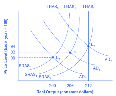
Figure 1 uses an aggregate demand/aggregate supply diagram to illustrate a healthy, growing economy. The original equilibrium occurs at E₀, the intersection of aggregate demand curve AD₀ and aggregate supply curve AS₀, at an output level of 200 and a price level of 90.

One year later, aggregate supply has shifted to the right to AS₁ in the process of long-term economic growth, and aggregate demand has also shifted to the right to AD₁, keeping the economy operating at the new level of potential GDP. The new equilibrium (E₁) is at an output level of 206 and a price level of 92. One more year later, aggregate supply has again shifted to the right, now to AS₂, and aggregate demand shifts right as well to AD₂. Now the equilibrium is E₂, with an output level of 212 and a price level of 94. In short, the figure shows an economy that is growing steadily year to year, producing at its potential GDP each year, with only small inflationary increases in the price level.

The graph shows three aggregate supply curves, three aggregate demand curves, and three potential GDP lines. Each aggregate demand curve intersects with an aggregate supply curve and the potential GDP line.

Figure 1. A Healthy, Growing Economy. In this well-functioning economy, each year aggregate supply and aggregate demand shift to the right so that the economy proceeds from equilibrium E₀ to E₁ to E₂. Each year, the economy produces at potential GDP with only a small inflationary increase in the price level. But if aggregate demand does not smoothly shift to the right and match increases in aggregate supply, growth with deflation can develop.

In the real world, however, aggregate demand and aggregate supply do not always move neatly together, especially over short periods of time. Aggregate demand may fail to grow as fast as aggregate supply, or it may even decline causing a recession. This could be caused by a number of possible reasons: households become hesitant about consuming; firms decide against investing as much; or perhaps the demand from other countries for exports diminishes. For example, investment by private firms in physical capital in the U.S. economy boomed during the late 1990s, rising from 14.1% of GDP in 1993 to 17.2% in 2000, before falling back to 15.2% by 2002. Conversely, increases in aggregate demand could run ahead of increases in aggregate supply, causing inflationary increases in the price level. Business cycles of recession and boom are the consequence of shifts in aggregate supply and aggregate demand. As these occur, the government may choose to use fiscal policy to address the difference.

Expansionary Fiscal Policy

Expansionary fiscal policy increases the level of aggregate demand, through either increases in government spending or reductions in taxes. Expansionary policy can do this by:

increasing consumption by raising disposable income through cuts in personal income taxes or payroll taxes;
increasing investments by raising after-tax profits through cuts in business taxes; and
increasing government purchases through increased spending by the federal government on final goods and services and raising federal grants to state and local governments to increase their expenditures on final goods and services.

Contractionary fiscal policy does the reverse: it decreases the level of aggregate demand by decreasing consumption, decreasing investments, and decreasing government spending, either through cuts in government spending or increases in taxes. The aggregate demand/aggregate supply model is useful in judging whether expansionary or contractionary fiscal policy is appropriate.

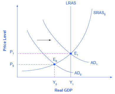
Consider first the situation in Figure 2, which is similar to the U.S. economy during the recession in 2008–2009. The intersection of aggregate demand (AD₀) and aggregate supply (AS₀) is occurring below the level of potential GDP. At the equilibrium (E₀), a recession occurs and unemployment rises. (The figure uses the upward-sloping AS curve associated with a Keynesian economic approach, rather than the vertical AS curve associated with a neoclassical approach, because our focus is on macroeconomic policy over the short-run business cycle rather than over the long run.) In this case, expansionary fiscal policy using tax cuts or increases in government spending can shift aggregate demand to AD₁, closer to the full-employment level of output. In addition, the price level would rise back to the level P₁ associated with potential GDP.

The graph shows two aggregate demand curves that each intersect with an aggregate supply curve. Aggregate demand curve (AD sub 1) intersects with both the aggregate supply curve (AS sub 0) as well as the potential GDP line.

Figure 2. Expansionary Fiscal Policy. The original equilibrium (E₀) represents a recession, occurring at a quantity of output (Yr) below potential GDP. However, a shift of aggregate demand from AD₀ to AD₁, enacted through an expansionary fiscal policy, can move the economy to a new equilibrium output of E₁ at the level of potential GDP. Since the economy was originally producing below potential GDP, any inflationary increase in the price level from P₀ to P₁ that results should be relatively small.

Should the government use tax cuts or spending increases, or a mix of the two, to carry out expansionary fiscal policy? After the Great Recession of 2008–2009, U.S. government spending rose from 19.6% of GDP in 2007 to 24.6% in 2009, while tax revenues declined from 18.5% of GDP in 2007 to 14.8% in 2009.

This very large budget deficit was produced by a combination of automatic stabilizers and discretionary fiscal policy. The Great Recession meant less tax-generating economic activity, which triggered the automatic stabilizers that reduce taxes. Most economists, even those who are concerned about a possible pattern of persistently large budget deficits, are much less concerned or even quite supportive of larger budget deficits in the short run of a few years during and immediately after a severe recession.

The Politics of Expansionary Fiscal Policy

The choice between whether to use tax or spending tools often has a political tinge. As a general statement, conservatives and Republicans prefer to see expansionary fiscal policy carried out by tax cuts, while liberals and Democrats prefer that expansionary fiscal policy be implemented through spending increases. The Obama administration and Congress passed an $830 billion expansionary policy in early 2009 involving both tax cuts and increases in government spending, according to the Congressional Budget Office. However, state and local governments, whose budgets were also hard hit by the recession, began cutting their spending—a policy that offset federal expansionary policy.

The conflict over which policy tool to use can be frustrating to those who want to categorize economics as “liberal” or “conservative,” or who want to use economic models to argue against their political opponents. But the AD–AS model can be used both by advocates of smaller government, who seek to reduce taxes and government spending, and by advocates of bigger government, who seek to raise taxes and government spending. Economic studies of specific taxing and spending programs can help to inform decisions about whether taxes or spending should be changed, and in what ways. Ultimately, decisions about whether to use tax or spending mechanisms to implement macroeconomic policy is, in part, a political decision rather than a purely economic one.

Try It

https://assessments.lumenlearning.co...sessments/7589

Watch It

A link to an interactive elements can be found at the bottom of this page.

Contractionary Fiscal Policy

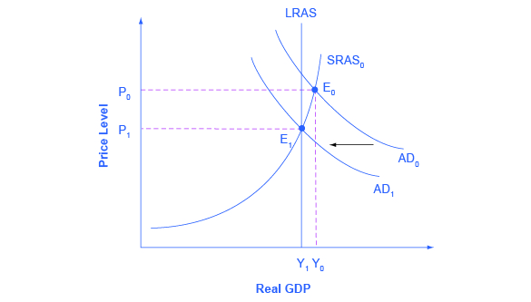
Fiscal policy can also be used to slow down an overheating economy. Suppose the macro equilibrium occurs at a level of GDP above potential, as shown in Figure 3. The intersection of aggregate demand (AD₀) and aggregate supply (AS₀) occurs at equilibrium E_0.In this situation, contractionary fiscal policy involving federal spending cuts or tax increases can help to reduce the upward pressure on the price level by shifting aggregate demand to the left, to AD₁, and causing the new equilibrium E₁ to be at potential GDP.

Figure 3. A Contractionary Fiscal Policy. The economy starts at the equilibrium quantity of output Yr, which is above potential GDP. The extremely high level of aggregate demand will generate inflationary increases in the price level. A contractionary fiscal policy can shift aggregate demand down from AD₀ to AD₁, leading to a new equilibrium output E₁, which occurs at potential GDP.

Again, the AD–AS model does not dictate how this contractionary fiscal policy is to be carried out. Some may prefer spending cuts; others may prefer tax increases; still others may say that it depends on the specific situation. The model only argues that, in this situation, aggregate demand needs to be reduced.

Try It

https://assessments.lumenlearning.co...sessments/7590

Learning Objectives

Contributors and Attributions

Modification, adaptation, and original content. Provided by: Lumen Learning. License: CC BY: Attribution

Using Fiscal Policy to Fight Recession, Unemployment, and Inflation. Authored by: OpenStax College. Located at: https://cnx.org/contents/vEmOH-_p@4.44:T6rLOl1i@4/Using-Fiscal-Policy-to-Fight-R. License: CC BY: Attribution. License Terms: Download for free at http://cnx.org/contents/bc498e1f-efe...69ad09a82@4.44

Types of Fiscal Policy. Provided by: You Will Love Economics. Located at: https://www.youtube.com/watch?v=q-j8AUCLKgw. License: Other. License Terms: Standard YouTube License

Search

Text Color

Text Size

Margin Size

Font Type

Expansionary Fiscal Policy

The Politics of Expansionary Fiscal Policy

Contractionary Fiscal Policy