Business LibreTexts

9.12: Keynesian Economic Policy

  • Page ID
    47416
  • \( \newcommand{\vecs}[1]{\overset { \scriptstyle \rightharpoonup} {\mathbf{#1}} } \)

    \( \newcommand{\vecd}[1]{\overset{-\!-\!\rightharpoonup}{\vphantom{a}\smash {#1}}} \)

    \( \newcommand{\id}{\mathrm{id}}\) \( \newcommand{\Span}{\mathrm{span}}\)

    ( \newcommand{\kernel}{\mathrm{null}\,}\) \( \newcommand{\range}{\mathrm{range}\,}\)

    \( \newcommand{\RealPart}{\mathrm{Re}}\) \( \newcommand{\ImaginaryPart}{\mathrm{Im}}\)

    \( \newcommand{\Argument}{\mathrm{Arg}}\) \( \newcommand{\norm}[1]{\| #1 \|}\)

    \( \newcommand{\inner}[2]{\langle #1, #2 \rangle}\)

    \( \newcommand{\Span}{\mathrm{span}}\)

    \( \newcommand{\id}{\mathrm{id}}\)

    \( \newcommand{\Span}{\mathrm{span}}\)

    \( \newcommand{\kernel}{\mathrm{null}\,}\)

    \( \newcommand{\range}{\mathrm{range}\,}\)

    \( \newcommand{\RealPart}{\mathrm{Re}}\)

    \( \newcommand{\ImaginaryPart}{\mathrm{Im}}\)

    \( \newcommand{\Argument}{\mathrm{Arg}}\)

    \( \newcommand{\norm}[1]{\| #1 \|}\)

    \( \newcommand{\inner}[2]{\langle #1, #2 \rangle}\)

    \( \newcommand{\Span}{\mathrm{span}}\) \( \newcommand{\AA}{\unicode[.8,0]{x212B}}\)

    \( \newcommand{\vectorA}[1]{\vec{#1}}      % arrow\)

    \( \newcommand{\vectorAt}[1]{\vec{\text{#1}}}      % arrow\)

    \( \newcommand{\vectorB}[1]{\overset { \scriptstyle \rightharpoonup} {\mathbf{#1}} } \)

    \( \newcommand{\vectorC}[1]{\textbf{#1}} \)

    \( \newcommand{\vectorD}[1]{\overrightarrow{#1}} \)

    \( \newcommand{\vectorDt}[1]{\overrightarrow{\text{#1}}} \)

    \( \newcommand{\vectE}[1]{\overset{-\!-\!\rightharpoonup}{\vphantom{a}\smash{\mathbf {#1}}}} \)

    \( \newcommand{\vecs}[1]{\overset { \scriptstyle \rightharpoonup} {\mathbf{#1}} } \)

    \( \newcommand{\vecd}[1]{\overset{-\!-\!\rightharpoonup}{\vphantom{a}\smash {#1}}} \)

    \(\newcommand{\avec}{\mathbf a}\) \(\newcommand{\bvec}{\mathbf b}\) \(\newcommand{\cvec}{\mathbf c}\) \(\newcommand{\dvec}{\mathbf d}\) \(\newcommand{\dtil}{\widetilde{\mathbf d}}\) \(\newcommand{\evec}{\mathbf e}\) \(\newcommand{\fvec}{\mathbf f}\) \(\newcommand{\nvec}{\mathbf n}\) \(\newcommand{\pvec}{\mathbf p}\) \(\newcommand{\qvec}{\mathbf q}\) \(\newcommand{\svec}{\mathbf s}\) \(\newcommand{\tvec}{\mathbf t}\) \(\newcommand{\uvec}{\mathbf u}\) \(\newcommand{\vvec}{\mathbf v}\) \(\newcommand{\wvec}{\mathbf w}\) \(\newcommand{\xvec}{\mathbf x}\) \(\newcommand{\yvec}{\mathbf y}\) \(\newcommand{\zvec}{\mathbf z}\) \(\newcommand{\rvec}{\mathbf r}\) \(\newcommand{\mvec}{\mathbf m}\) \(\newcommand{\zerovec}{\mathbf 0}\) \(\newcommand{\onevec}{\mathbf 1}\) \(\newcommand{\real}{\mathbb R}\) \(\newcommand{\twovec}[2]{\left[\begin{array}{r}#1 \\ #2 \end{array}\right]}\) \(\newcommand{\ctwovec}[2]{\left[\begin{array}{c}#1 \\ #2 \end{array}\right]}\) \(\newcommand{\threevec}[3]{\left[\begin{array}{r}#1 \\ #2 \\ #3 \end{array}\right]}\) \(\newcommand{\cthreevec}[3]{\left[\begin{array}{c}#1 \\ #2 \\ #3 \end{array}\right]}\) \(\newcommand{\fourvec}[4]{\left[\begin{array}{r}#1 \\ #2 \\ #3 \\ #4 \end{array}\right]}\) \(\newcommand{\cfourvec}[4]{\left[\begin{array}{c}#1 \\ #2 \\ #3 \\ #4 \end{array}\right]}\) \(\newcommand{\fivevec}[5]{\left[\begin{array}{r}#1 \\ #2 \\ #3 \\ #4 \\ #5 \\ \end{array}\right]}\) \(\newcommand{\cfivevec}[5]{\left[\begin{array}{c}#1 \\ #2 \\ #3 \\ #4 \\ #5 \\ \end{array}\right]}\) \(\newcommand{\mattwo}[4]{\left[\begin{array}{rr}#1 \amp #2 \\ #3 \amp #4 \\ \end{array}\right]}\) \(\newcommand{\laspan}[1]{\text{Span}\{#1\}}\) \(\newcommand{\bcal}{\cal B}\) \(\newcommand{\ccal}{\cal C}\) \(\newcommand{\scal}{\cal S}\) \(\newcommand{\wcal}{\cal W}\) \(\newcommand{\ecal}{\cal E}\) \(\newcommand{\coords}[2]{\left\{#1\right\}_{#2}}\) \(\newcommand{\gray}[1]{\color{gray}{#1}}\) \(\newcommand{\lgray}[1]{\color{lightgray}{#1}}\) \(\newcommand{\rank}{\operatorname{rank}}\) \(\newcommand{\row}{\text{Row}}\) \(\newcommand{\col}{\text{Col}}\) \(\renewcommand{\row}{\text{Row}}\) \(\newcommand{\nul}{\text{Nul}}\) \(\newcommand{\var}{\text{Var}}\) \(\newcommand{\corr}{\text{corr}}\) \(\newcommand{\len}[1]{\left|#1\right|}\) \(\newcommand{\bbar}{\overline{\bvec}}\) \(\newcommand{\bhat}{\widehat{\bvec}}\) \(\newcommand{\bperp}{\bvec^\perp}\) \(\newcommand{\xhat}{\widehat{\xvec}}\) \(\newcommand{\vhat}{\widehat{\vvec}}\) \(\newcommand{\uhat}{\widehat{\uvec}}\) \(\newcommand{\what}{\widehat{\wvec}}\) \(\newcommand{\Sighat}{\widehat{\Sigma}}\) \(\newcommand{\lt}{<}\) \(\newcommand{\gt}{>}\) \(\newcommand{\amp}{&}\) \(\definecolor{fillinmathshade}{gray}{0.9}\)

    Learning Objectives

    • Describe the GDP gap
    • Explain the Keynesian logic for expansionary and contractionary fiscal policy for reducing unemployment and inflation

    The GDP Gap

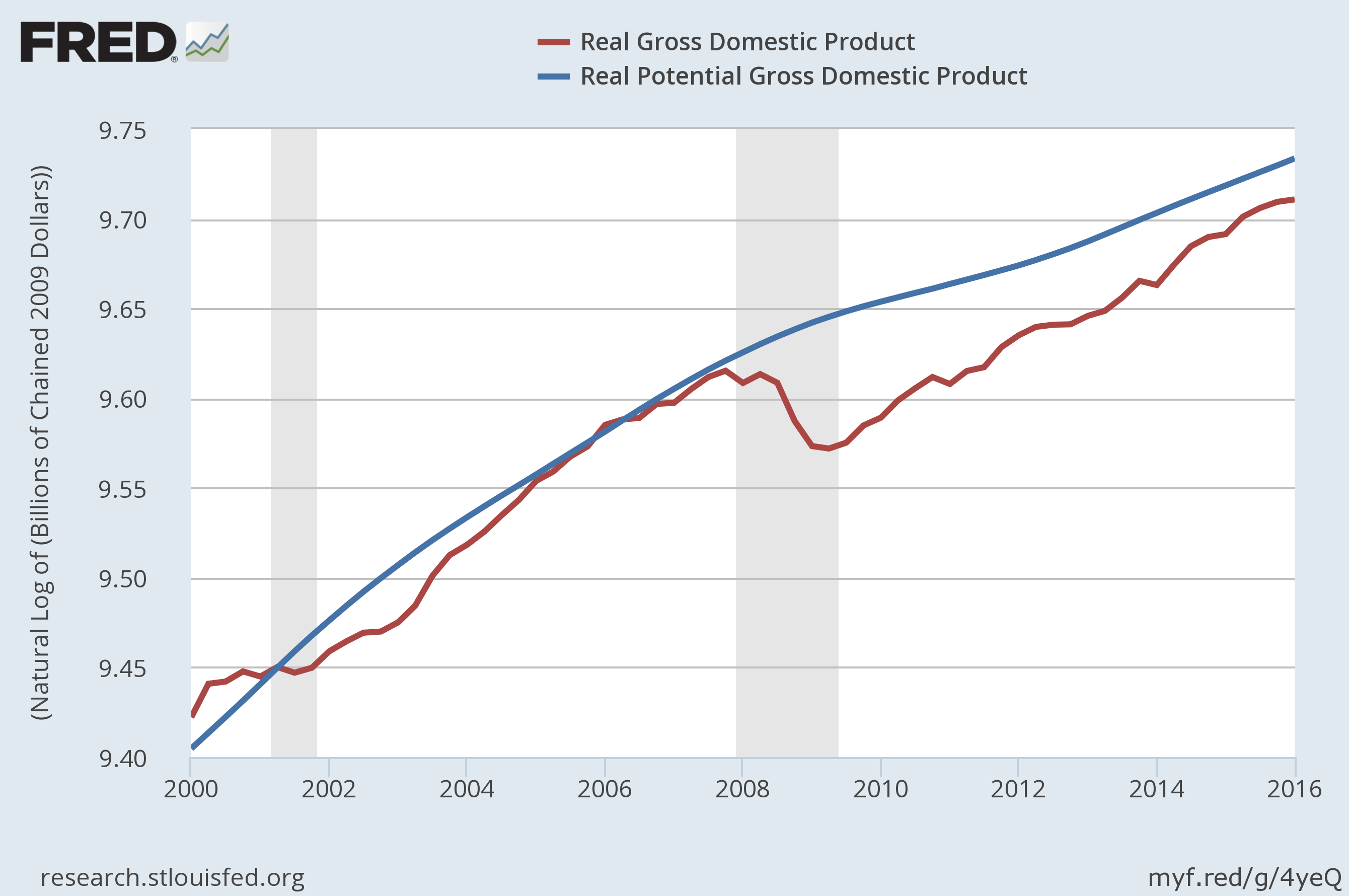
    The GDP gap is defined as the difference between potential GDP and actual GDP, when both are measured in real terms. When the economy falls into recession, the GDP gap is positive, meaning the economy is operating at less than potential (and less than full employment). When the economy experiences an inflationary boom, the GDP gap is negative, meaning the economy is operating at greater than potential (and more than full employment).

    Line graph showing real GDP and potential GDP between 2000 and 2016. The lines stay close through many of the years, but in 2001, real GDP falls behind and takes 5 years to recover, then real GDP falls again in 20018 and has not yet recovered by 2016.
    Figure 1. The GDP Gap. Potential (blue) and actual (red) GDP estimates from the Congressional Budget Office (CBO). The difference between the two lines is the GDP gap. The gray columns show areas of recession.

    Since the neoclassical model assumes the economy operates at (exactly) full employment, the GDP Gap isn’t really relevant to Neoclassical analysis but it is integral to the Keynesian view of the world, as we describe next.

    Keynesian Policy for Fighting Unemployment and Inflation

    Keynesian economists argue that since the level of economic activity depends on aggregate demand, but that aggregate demand can’t be counted on to stay at potential real GDP, the economy is likely to be characterized by recessions and inflationary booms. This cycle can be seen as fluctuations between positive and negative GDP gaps.

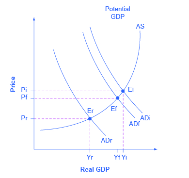
    Keynesians believe that the solution to a recession is expansionary fiscal policy, such as tax cuts to stimulate consumption and investment, or direct increases in government spending, either of which would shift the aggregate demand curve to the right. For example, if aggregate demand was originally at ADr in Figure 2, so that the economy was in recession, the appropriate policy would be for government to shift aggregate demand to the right from ADr to ADf, where the economy would be at potential GDP and full employment.

    Keynes noted that while it would be nice if the government could spend additional money on housing, roads, and other public goods, he also argued that if the government could not agree on how to spend money in practical ways, then it could spend in impractical ways. For example, Keynes suggested building monuments, like a modern equivalent of the Egyptian pyramids. He proposed that the government could bury money underground, and let mining companies get started to dig the money up again. While these suggestions were tongue-in-cheek, their purpose was to emphasize that a Great Depression is no time to quibble over the specifics of government spending programs and tax cuts when the goal should be to pump up aggregate demand by enough to lift the economy to potential GDP.

    The graph shows three possible downward-sloping AD curves, an upward-sloping AS curve, and a vertical, straight potential GDP line.
    Figure 2. Fighting Recession and Inflation with Keynesian Policy. If an economy is in recession, with an equilibrium at Er, then the Keynesian response would be to enact a policy to shift aggregate demand to the right from ADr toward ADf. If an economy is experiencing inflationary pressures with an equilibrium at Ei, then the Keynesian response would be to enact a policy response to shift aggregate demand to the left, from ADi toward ADf.

    The other side of Keynesian policy occurs when the economy is operating above potential GDP. In this situation, unemployment is low, but inflationary rises in the price level are a concern. The Keynesian response would be contractionary fiscal policy, using tax increases or government spending cuts to shift AD to the left. The result would be downward pressure on the price level, but very little reduction in output or very little rise in unemployment. If aggregate demand was originally at ADi in Figure 2, so that the economy was experiencing inflationary rises in the price level, the appropriate policy would be for government to shift aggregate demand to the left, from ADi toward ADf, which reduces the pressure for a higher price level while the economy remains at full employment.

    In the Keynesian economic model, too little aggregate demand brings unemployment and too much brings inflation. Thus, you can think of Keynesian economics as pursuing a “Goldilocks” level of aggregate demand: not too much, not too little, but looking for what is just right.

    The Keynesian Perspective on Market Forces

    Ever since the birth of Keynesian economics in the 1930s, controversy has simmered over the extent to which government should play an active role in managing the economy. In the aftermath of the human devastation and misery of the Great Depression, many people—including many economists—became more aware of vulnerabilities within the market-oriented economic system.

    However, Keynes himself was careful to separate the issue of aggregate demand from the issue of how well individual markets worked. He argued that individual markets for goods and services were appropriate and useful, but that sometimes that level of aggregate demand was just too low. When 10 million people are willing and able to work, but one million of them are unemployed, he argued, individual markets may be doing a perfectly good job of allocating the efforts of the nine million workers—the problem is that insufficient aggregate demand exists to support jobs for all 10 million. Thus, he believed that, while government should ensure that overall level of aggregate demand is sufficient for an economy to reach full employment, this task did not imply that the government should attempt to set prices and wages throughout the economy, nor to take over and manage large corporations or entire industries directly.

    The Keynesian approach, with its focus on aggregate demand and sticky prices, has proved useful in understanding how the economy fluctuates in the short run and why recessions and cyclical unemployment occur. Later, will we cover a different viewpoint—the neoclassical perspective—and will consider some of the shortcomings of the Keynesian approach and why it is not especially well-suited for long-run macroeconomic analysis.

    THE GREAT RECESSION

    The lessons learned during the Great Depression of the 1930s and the aggregate expenditure model proposed by John Maynard Keynes gave the modern economists and policymakers of today the tools to effectively navigate the treacherous economy in the latter half of the 2000s. In “How the Great Recession Was Brought to an End,” Alan S. Blinder and Mark Zandi wrote that the actions taken by today’s policymakers stand in sharp contrast to those of the early years of the Great Depression. Today’s economists and policymakers were not content to let the markets recover from recession without taking proactive measures to support consumption and investment. The Federal Reserve actively lowered short-term interest rates and developed innovative ways to pump money into the economy so that credit and investment would not dry up. Both Presidents Bush and Obama (along with Congress) implemented a variety of programs ranging from tax rebates to “Cash for Clunkers” to the Troubled Asset Relief Program to stimulate and stabilize household consumption and encourage investment. Although these policies came under harsh criticism from the public and many politicians, they lessened the impact of the economic downturn and may have saved the country from a second Great Depression.

    Try It

    This question allows you to get as much practice as you need, as you can click the link at the top of the question (“Try another version of this question”) to get a new version of the question. Practice until you feel comfortable doing the question.

    [ohm_question]152988[/ohm_question]

    Try It

    This question allows you to get as much practice as you need, as you can click the link at the top of the question (“Try another version of this question”) to get a new version of the question. Practice until you feel comfortable doing the question.

    [ohm_question]153122[/ohm_question]


    Glossary

    [glossary-page][glossary-term]contractionary fiscal policy: [/glossary-term][glossary-definition]efforts to decrease aggregate demand through tax increases or government spending cuts[/glossary-definition]
    [glossary-term]expansionary fiscal policy:[/glossary-term][glossary-definition] efforts to increase aggregate demand through means such as tax cuts to stimulate consumption and investment, or direct increases in government spending[/glossary-definition][glossary-term]GDP gap: [/glossary-term][glossary-definition]The difference between actual and potential real GDP; during recessions the gap grows; during booms the gap becomes negative[/glossary-definition][/glossary-page]

    CC licensed content, Shared previously

    9.12: Keynesian Economic Policy is shared under a not declared license and was authored, remixed, and/or curated by LibreTexts.

    • Was this article helpful?