
14.12: The Demand for Labor
- Page ID
- 48486
\( \newcommand{\vecs}[1]{\overset { \scriptstyle \rightharpoonup} {\mathbf{#1}} } \)
\( \newcommand{\vecd}[1]{\overset{-\!-\!\rightharpoonup}{\vphantom{a}\smash {#1}}} \)
\( \newcommand{\id}{\mathrm{id}}\) \( \newcommand{\Span}{\mathrm{span}}\)
( \newcommand{\kernel}{\mathrm{null}\,}\) \( \newcommand{\range}{\mathrm{range}\,}\)
\( \newcommand{\RealPart}{\mathrm{Re}}\) \( \newcommand{\ImaginaryPart}{\mathrm{Im}}\)
\( \newcommand{\Argument}{\mathrm{Arg}}\) \( \newcommand{\norm}[1]{\| #1 \|}\)
\( \newcommand{\inner}[2]{\langle #1, #2 \rangle}\)
\( \newcommand{\Span}{\mathrm{span}}\)
\( \newcommand{\id}{\mathrm{id}}\)
\( \newcommand{\Span}{\mathrm{span}}\)
\( \newcommand{\kernel}{\mathrm{null}\,}\)
\( \newcommand{\range}{\mathrm{range}\,}\)
\( \newcommand{\RealPart}{\mathrm{Re}}\)
\( \newcommand{\ImaginaryPart}{\mathrm{Im}}\)
\( \newcommand{\Argument}{\mathrm{Arg}}\)
\( \newcommand{\norm}[1]{\| #1 \|}\)
\( \newcommand{\inner}[2]{\langle #1, #2 \rangle}\)
\( \newcommand{\Span}{\mathrm{span}}\) \( \newcommand{\AA}{\unicode[.8,0]{x212B}}\)
\( \newcommand{\vectorA}[1]{\vec{#1}} % arrow\)
\( \newcommand{\vectorAt}[1]{\vec{\text{#1}}} % arrow\)
\( \newcommand{\vectorB}[1]{\overset { \scriptstyle \rightharpoonup} {\mathbf{#1}} } \)
\( \newcommand{\vectorC}[1]{\textbf{#1}} \)
\( \newcommand{\vectorD}[1]{\overrightarrow{#1}} \)
\( \newcommand{\vectorDt}[1]{\overrightarrow{\text{#1}}} \)
\( \newcommand{\vectE}[1]{\overset{-\!-\!\rightharpoonup}{\vphantom{a}\smash{\mathbf {#1}}}} \)
\( \newcommand{\vecs}[1]{\overset { \scriptstyle \rightharpoonup} {\mathbf{#1}} } \)
\( \newcommand{\vecd}[1]{\overset{-\!-\!\rightharpoonup}{\vphantom{a}\smash {#1}}} \)
\(\newcommand{\avec}{\mathbf a}\) \(\newcommand{\bvec}{\mathbf b}\) \(\newcommand{\cvec}{\mathbf c}\) \(\newcommand{\dvec}{\mathbf d}\) \(\newcommand{\dtil}{\widetilde{\mathbf d}}\) \(\newcommand{\evec}{\mathbf e}\) \(\newcommand{\fvec}{\mathbf f}\) \(\newcommand{\nvec}{\mathbf n}\) \(\newcommand{\pvec}{\mathbf p}\) \(\newcommand{\qvec}{\mathbf q}\) \(\newcommand{\svec}{\mathbf s}\) \(\newcommand{\tvec}{\mathbf t}\) \(\newcommand{\uvec}{\mathbf u}\) \(\newcommand{\vvec}{\mathbf v}\) \(\newcommand{\wvec}{\mathbf w}\) \(\newcommand{\xvec}{\mathbf x}\) \(\newcommand{\yvec}{\mathbf y}\) \(\newcommand{\zvec}{\mathbf z}\) \(\newcommand{\rvec}{\mathbf r}\) \(\newcommand{\mvec}{\mathbf m}\) \(\newcommand{\zerovec}{\mathbf 0}\) \(\newcommand{\onevec}{\mathbf 1}\) \(\newcommand{\real}{\mathbb R}\) \(\newcommand{\twovec}[2]{\left[\begin{array}{r}#1 \\ #2 \end{array}\right]}\) \(\newcommand{\ctwovec}[2]{\left[\begin{array}{c}#1 \\ #2 \end{array}\right]}\) \(\newcommand{\threevec}[3]{\left[\begin{array}{r}#1 \\ #2 \\ #3 \end{array}\right]}\) \(\newcommand{\cthreevec}[3]{\left[\begin{array}{c}#1 \\ #2 \\ #3 \end{array}\right]}\) \(\newcommand{\fourvec}[4]{\left[\begin{array}{r}#1 \\ #2 \\ #3 \\ #4 \end{array}\right]}\) \(\newcommand{\cfourvec}[4]{\left[\begin{array}{c}#1 \\ #2 \\ #3 \\ #4 \end{array}\right]}\) \(\newcommand{\fivevec}[5]{\left[\begin{array}{r}#1 \\ #2 \\ #3 \\ #4 \\ #5 \\ \end{array}\right]}\) \(\newcommand{\cfivevec}[5]{\left[\begin{array}{c}#1 \\ #2 \\ #3 \\ #4 \\ #5 \\ \end{array}\right]}\) \(\newcommand{\mattwo}[4]{\left[\begin{array}{rr}#1 \amp #2 \\ #3 \amp #4 \\ \end{array}\right]}\) \(\newcommand{\laspan}[1]{\text{Span}\{#1\}}\) \(\newcommand{\bcal}{\cal B}\) \(\newcommand{\ccal}{\cal C}\) \(\newcommand{\scal}{\cal S}\) \(\newcommand{\wcal}{\cal W}\) \(\newcommand{\ecal}{\cal E}\) \(\newcommand{\coords}[2]{\left\{#1\right\}_{#2}}\) \(\newcommand{\gray}[1]{\color{gray}{#1}}\) \(\newcommand{\lgray}[1]{\color{lightgray}{#1}}\) \(\newcommand{\rank}{\operatorname{rank}}\) \(\newcommand{\row}{\text{Row}}\) \(\newcommand{\col}{\text{Col}}\) \(\renewcommand{\row}{\text{Row}}\) \(\newcommand{\nul}{\text{Nul}}\) \(\newcommand{\var}{\text{Var}}\) \(\newcommand{\corr}{\text{corr}}\) \(\newcommand{\len}[1]{\left|#1\right|}\) \(\newcommand{\bbar}{\overline{\bvec}}\) \(\newcommand{\bhat}{\widehat{\bvec}}\) \(\newcommand{\bperp}{\bvec^\perp}\) \(\newcommand{\xhat}{\widehat{\xvec}}\) \(\newcommand{\vhat}{\widehat{\vvec}}\) \(\newcommand{\uhat}{\widehat{\uvec}}\) \(\newcommand{\what}{\widehat{\wvec}}\) \(\newcommand{\Sighat}{\widehat{\Sigma}}\) \(\newcommand{\lt}{<}\) \(\newcommand{\gt}{>}\) \(\newcommand{\amp}{&}\) \(\definecolor{fillinmathshade}{gray}{0.9}\)Learning Objectives
- Explain and graph the demand for labor in perfectly competitive output markets
- Explain and graph the demand for labor in imperfectly competitive output markets
- Demonstrate how supply and demand interact to determine the market wage rate
Demand for Labor in Perfectly Competitive Output Markets
The question for any firm is how much labor to hire.
We can define a perfectly competitive labor market as one where firms can hire all the labor they wish at the going market wage. Think about secretaries in a large city. Employers who need secretaries can probably hire as many as they need if they pay the going wage rate.
Graphically, this means that firms face a horizontal supply curve for labor, as Figure 1 shows.
Given the market wage, profit maximizing firms hire workers up to the point where: Wmkt = VMPL

Derived Demand
Economists describe the demand for inputs like labor as a derived demand. Since the demand for labor is MPL*P, it is dependent on the demand for the product the firm is producing. We show this by the P term in the demand for labor. An increase in demand for the firm’s product drives up the product’s price, which increases the firm’s demand for labor. Thus, we derive the demand for labor from the demand for the firm’s output.
Demand for Labor in Imperfectly Competitive Output Markets
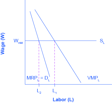
If an employer does not sell its output in a perfectly competitive industry, it faces a downward sloping demand curve for output. This means that in order to sell additional output the firm must lower its price. This is true if the firm is a monopoly, but it’s also true if the firm is an oligopoly or monopolistically competitive. In this situation, the value of an additional unit of output sold is the marginal revenue, rather than the price. This means that a worker’s marginal product is valued by the marginal revenue, not the price. Thus, the demand for labor is the marginal product times the marginal revenue, which we call the marginal revenue product.
The Demand for Labor = MPL x MR = Marginal Revenue Product
| # Workers (L) | 1 | 2 | 3 | 4 |
| MPL | 4 | 3 | 2 | 1 |
| Marginal Revenue | $4 | $3 | $2 | $1 |
| MRPL | $16 | $9 | $4 | $1 |

Everything else remains the same as we described above in the discussion of the labor demand in perfectly competitive labor markets. Given the market wage, profit-maximizing firms will hire workers up to the point where the market wage equals the marginal revenue product, as Figure 3 shows.
Do Profit-Maximizing Employers Exploit Labor?
If you look back at Figure 3, you will see that the firm only pays the last worker it hires what they’re worth to the firm. Every other worker brings in more revenue than the firm pays him or her. This has sometimes led to the claim that employers exploit workers because they do not pay workers what they are worth. Let’s think about this claim. The first worker is worth $x to the firm, and the second worker is worth $y, but why are they worth that much? It is because of the capital and technology with which they work. The difference between workers’ worth and their compensation goes to pay for the capital, and other inputs in the production process. The difference also goes to the employer’s profit, without which the firm would close and workers wouldn’t have a job. The firm may be earning excessive profits, but that is a different topic of discussion.
What Determines the Going Market Wage Rate?
We learned earlier that the labor market has demand and supply curves like other markets. The demand for labor curve is a downward sloping function of the wage rate. The market demand for labor is the horizontal sum of all firms’ demands for labor. The supply for labor curve is an upward sloping function of the wage rate. This is because if wages for a particular type of labor increase in a particular labor market, people with appropriate skills may change jobs, and vacancies will attract people from outside the geographic area. The market supply for labor is the horizontal summation of all individuals’ supplies of labor.

Like all equilibrium prices, the market wage rate is determined through the interaction of supply and demand in the labor market. Thus, we can see in Figure 4, the wage rate and number of workers hired in a competitive labor market.
Watch It
Watch this video for a nice overview of the labor market, and the ways that supply and demand interact to determine wages. The video will also introduce some of the key concepts we’ll discuss soon, including monopsonies, unions, discrimination, and minimum wage laws.
Learning Objectives
[glossary-page][glossary-term]collective bargaining:[/glossary-term]
[glossary-definition]negotiations between unions and a firm or firms[/glossary-definition][glossary-term]labor union:[/glossary-term]
[glossary-definition]an organization of workers that negotiates with employers over wages and working conditions[/glossary-definition][glossary-term]perfectly competitive labor market:[/glossary-term]
[glossary-definition]a labor market where neither suppliers of labor nor demanders of labor have any market power; thus, an employer can hire all the workers they would like at the going market wage[/glossary-definition][glossary-term]marginal revenue product of labor:[/glossary-term]
[glossary-definition]the marginal product of an additional worker multiplied by the marginal revenue to the firm of the additional worker’s output[/glossary-definition][/glossary-page]
Contributors and Attributions
- The Theory of Labor Markets. Authored by: OpenStax College. Located at: https://cnx.org/contents/vEmOH-_p@4.41:QsI0grBK/The-Theory-of-Labor-Markets. License: CC BY: Attribution. License Terms: Download for free at http://cnx.org/contents/bc498e1f-efe...569ad09a82@4.4
- Labor Markets and Minimum Wage: Crash Course Economics #28. Provided by: CrashCourse. Located at: https://www.youtube.com/watch?v=mWwXmH-n5Bo. License: All Rights Reserved. License Terms: Standard YouTube License