
11.16: Profit Maximization for a Monopoly
- Page ID
- 48433
\( \newcommand{\vecs}[1]{\overset { \scriptstyle \rightharpoonup} {\mathbf{#1}} } \)
\( \newcommand{\vecd}[1]{\overset{-\!-\!\rightharpoonup}{\vphantom{a}\smash {#1}}} \)
\( \newcommand{\id}{\mathrm{id}}\) \( \newcommand{\Span}{\mathrm{span}}\)
( \newcommand{\kernel}{\mathrm{null}\,}\) \( \newcommand{\range}{\mathrm{range}\,}\)
\( \newcommand{\RealPart}{\mathrm{Re}}\) \( \newcommand{\ImaginaryPart}{\mathrm{Im}}\)
\( \newcommand{\Argument}{\mathrm{Arg}}\) \( \newcommand{\norm}[1]{\| #1 \|}\)
\( \newcommand{\inner}[2]{\langle #1, #2 \rangle}\)
\( \newcommand{\Span}{\mathrm{span}}\)
\( \newcommand{\id}{\mathrm{id}}\)
\( \newcommand{\Span}{\mathrm{span}}\)
\( \newcommand{\kernel}{\mathrm{null}\,}\)
\( \newcommand{\range}{\mathrm{range}\,}\)
\( \newcommand{\RealPart}{\mathrm{Re}}\)
\( \newcommand{\ImaginaryPart}{\mathrm{Im}}\)
\( \newcommand{\Argument}{\mathrm{Arg}}\)
\( \newcommand{\norm}[1]{\| #1 \|}\)
\( \newcommand{\inner}[2]{\langle #1, #2 \rangle}\)
\( \newcommand{\Span}{\mathrm{span}}\) \( \newcommand{\AA}{\unicode[.8,0]{x212B}}\)
\( \newcommand{\vectorA}[1]{\vec{#1}} % arrow\)
\( \newcommand{\vectorAt}[1]{\vec{\text{#1}}} % arrow\)
\( \newcommand{\vectorB}[1]{\overset { \scriptstyle \rightharpoonup} {\mathbf{#1}} } \)
\( \newcommand{\vectorC}[1]{\textbf{#1}} \)
\( \newcommand{\vectorD}[1]{\overrightarrow{#1}} \)
\( \newcommand{\vectorDt}[1]{\overrightarrow{\text{#1}}} \)
\( \newcommand{\vectE}[1]{\overset{-\!-\!\rightharpoonup}{\vphantom{a}\smash{\mathbf {#1}}}} \)
\( \newcommand{\vecs}[1]{\overset { \scriptstyle \rightharpoonup} {\mathbf{#1}} } \)
\( \newcommand{\vecd}[1]{\overset{-\!-\!\rightharpoonup}{\vphantom{a}\smash {#1}}} \)
\(\newcommand{\avec}{\mathbf a}\) \(\newcommand{\bvec}{\mathbf b}\) \(\newcommand{\cvec}{\mathbf c}\) \(\newcommand{\dvec}{\mathbf d}\) \(\newcommand{\dtil}{\widetilde{\mathbf d}}\) \(\newcommand{\evec}{\mathbf e}\) \(\newcommand{\fvec}{\mathbf f}\) \(\newcommand{\nvec}{\mathbf n}\) \(\newcommand{\pvec}{\mathbf p}\) \(\newcommand{\qvec}{\mathbf q}\) \(\newcommand{\svec}{\mathbf s}\) \(\newcommand{\tvec}{\mathbf t}\) \(\newcommand{\uvec}{\mathbf u}\) \(\newcommand{\vvec}{\mathbf v}\) \(\newcommand{\wvec}{\mathbf w}\) \(\newcommand{\xvec}{\mathbf x}\) \(\newcommand{\yvec}{\mathbf y}\) \(\newcommand{\zvec}{\mathbf z}\) \(\newcommand{\rvec}{\mathbf r}\) \(\newcommand{\mvec}{\mathbf m}\) \(\newcommand{\zerovec}{\mathbf 0}\) \(\newcommand{\onevec}{\mathbf 1}\) \(\newcommand{\real}{\mathbb R}\) \(\newcommand{\twovec}[2]{\left[\begin{array}{r}#1 \\ #2 \end{array}\right]}\) \(\newcommand{\ctwovec}[2]{\left[\begin{array}{c}#1 \\ #2 \end{array}\right]}\) \(\newcommand{\threevec}[3]{\left[\begin{array}{r}#1 \\ #2 \\ #3 \end{array}\right]}\) \(\newcommand{\cthreevec}[3]{\left[\begin{array}{c}#1 \\ #2 \\ #3 \end{array}\right]}\) \(\newcommand{\fourvec}[4]{\left[\begin{array}{r}#1 \\ #2 \\ #3 \\ #4 \end{array}\right]}\) \(\newcommand{\cfourvec}[4]{\left[\begin{array}{c}#1 \\ #2 \\ #3 \\ #4 \end{array}\right]}\) \(\newcommand{\fivevec}[5]{\left[\begin{array}{r}#1 \\ #2 \\ #3 \\ #4 \\ #5 \\ \end{array}\right]}\) \(\newcommand{\cfivevec}[5]{\left[\begin{array}{c}#1 \\ #2 \\ #3 \\ #4 \\ #5 \\ \end{array}\right]}\) \(\newcommand{\mattwo}[4]{\left[\begin{array}{rr}#1 \amp #2 \\ #3 \amp #4 \\ \end{array}\right]}\) \(\newcommand{\laspan}[1]{\text{Span}\{#1\}}\) \(\newcommand{\bcal}{\cal B}\) \(\newcommand{\ccal}{\cal C}\) \(\newcommand{\scal}{\cal S}\) \(\newcommand{\wcal}{\cal W}\) \(\newcommand{\ecal}{\cal E}\) \(\newcommand{\coords}[2]{\left\{#1\right\}_{#2}}\) \(\newcommand{\gray}[1]{\color{gray}{#1}}\) \(\newcommand{\lgray}[1]{\color{lightgray}{#1}}\) \(\newcommand{\rank}{\operatorname{rank}}\) \(\newcommand{\row}{\text{Row}}\) \(\newcommand{\col}{\text{Col}}\) \(\renewcommand{\row}{\text{Row}}\) \(\newcommand{\nul}{\text{Nul}}\) \(\newcommand{\var}{\text{Var}}\) \(\newcommand{\corr}{\text{corr}}\) \(\newcommand{\len}[1]{\left|#1\right|}\) \(\newcommand{\bbar}{\overline{\bvec}}\) \(\newcommand{\bhat}{\widehat{\bvec}}\) \(\newcommand{\bperp}{\bvec^\perp}\) \(\newcommand{\xhat}{\widehat{\xvec}}\) \(\newcommand{\vhat}{\widehat{\vvec}}\) \(\newcommand{\uhat}{\widehat{\uvec}}\) \(\newcommand{\what}{\widehat{\wvec}}\) \(\newcommand{\Sighat}{\widehat{\Sigma}}\) \(\newcommand{\lt}{<}\) \(\newcommand{\gt}{>}\) \(\newcommand{\amp}{&}\) \(\definecolor{fillinmathshade}{gray}{0.9}\)Learning Objectives
- Describe how a demand curve for a monopoly differs from a demand curve for a perfectly competitive firm
- Analyze total cost and total revenue curves for a monopolist
- Describe and calculate marginal revenue and marginal cost in a monopoly
- Determine the level of output the monopolist should supply and the price it should charge in order to maximize profit
Demand Curves Perceived by a Perfectly Competitive Firm and by a Monopoly
Consider a monopoly firm, comfortably surrounded by barriers to entry so that it need not fear competition from other producers. How will this monopoly choose its profit-maximizing quantity of output, and what price will it charge? Profits for the monopolist, like any firm, will be equal to total revenues minus total costs. The pattern of costs for the monopoly can be analyzed within the same framework as the costs of a perfectly competitive firm—that is, by using total cost, fixed cost, variable cost, marginal cost, average cost, and average variable cost. However, because a monopoly faces no competition, its situation and its decision process will differ from that of a perfectly competitive firm.
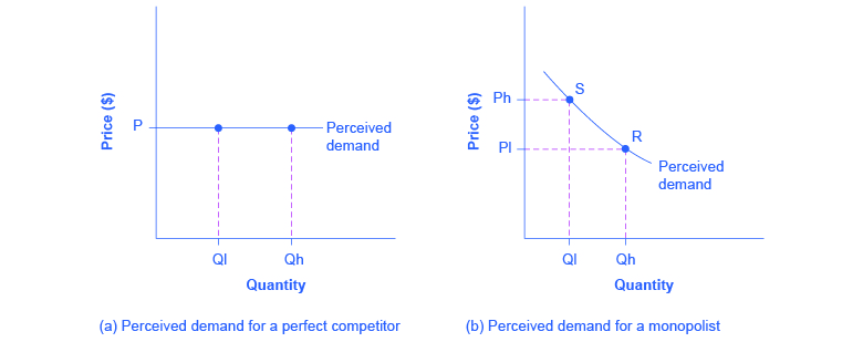
A perfectly competitive firm acts as a price taker. The demand curve it perceives appears in Figure 1(a). The horizontal demand curve means that, from the viewpoint of the perfectly competitive firm, it could sell either a relatively low quantity like Ql or a relatively high quantity like Qh at the market price P.
What Defines the Market?
A monopoly is a firm that sells all or nearly all of the goods and services in a given market. But what defines the “market”?
In a famous 1947 case, the federal government accused the DuPont company of having a monopoly in the cellophane market, pointing out that DuPont produced 75% of the cellophane in the United States. DuPont countered that even though it had a 75% market share in cellophane, it had less than a 20% share of the “flexible packaging materials,” which includes all other moisture-proof papers, films, and foils. In 1956, after years of legal appeals, the U.S. Supreme Court held that the broader market definition was more appropriate, and the case against DuPont was dismissed.
Questions over how to define the market continue today. True, Microsoft in the 1990s had a dominant share of the software for computer operating systems, but in the total market for all computer software and services, including everything from games to scientific programs, the Microsoft share was only about 16% in 2000. The Greyhound bus company may have a near-monopoly on the market for intercity bus transportation, but it is only a small share of the market for intercity transportation if that market includes private cars, airplanes, and railroad service. DeBeers has a monopoly in diamonds, but it is a much smaller share of the total market for precious gemstones and an even smaller share of the total market for jewelry. A small town in the country may have only one gas station: is this gas station a “monopoly,” or does it compete with gas stations that might be five, 10, or 50 miles away?
In general, if a firm produces a product without close substitutes, then the firm can be considered a monopoly producer in a single market. But if buyers have a range of similar—even if not identical—options available from other firms, then the firm is not a monopoly. Still, arguments over whether substitutes are close or not close can be controversial.
While a monopolist can charge any price for its product, that price is nonetheless constrained by demand for the firm’s product. No monopolist, even one that is thoroughly protected by high barriers to entry, can require consumers to purchase its product. Because the monopolist is the only firm in the market, its demand curve is the same as the market demand curve, which is, unlike that for a perfectly competitive firm, downward-sloping.
Figure 1 illustrates this situation. The monopolist can either choose a point like R with a low price (Pl) and high quantity (Qh), or a point like S with a high price (Ph) and a low quantity (Ql), or some intermediate point. Setting the price too high will result in a low quantity sold, and will not bring in much revenue. Conversely, setting the price too low may result in a high quantity sold, but because of the low price, it will not bring in much revenue either. The challenge for the monopolist is to strike a profit-maximizing balance between the price it charges and the quantity that it sells.
What is the Difference Between Perceived Demand and Market Demand?
The demand curve as perceived by a perfectly competitive firm is not the overall market demand curve for that product. However, the firm’s demand curve as perceived by a monopoly is the same as the market demand curve. The reason for the difference is that each perfectly competitive firm perceives the demand for its products in a market that includes many other firms; in effect, the demand curve perceived by a perfectly competitive firm is a tiny slice of the entire market demand curve. In contrast, a monopoly perceives demand for its product in a market where the monopoly is the only producer.
Total Cost and Total Revenue for a Monopolist
In order to determine profits for a monopolist, we need to first identify total revenues and total costs. An example for the hypothetical HealthPill firm is shown in Figure 2.
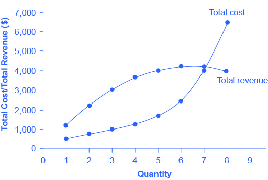
Total costs for a monopolist follow the same rules as for perfectly competitive firms. In other words, total costs increase with output at an increasing rate. Total revenue, by contrast, is different from perfect competition. Since a monopolist faces a downward sloping demand curve, the only way it can sell more output is by reducing its price. Selling more output raises revenue, but lowering price reduces it. Thus, the shape of total revenue isn’t clear. Let’s explore this using the data in Table 1, which shows points along the demand curve (quantity demanded and price), and then calculates total revenue by multiplying price times quantity. (In this example, we give the output as 1, 2, 3, 4, and so on, for the sake of simplicity. If you prefer a dash of greater realism, you can imagine that the pharmaceutical company measures these output levels and the corresponding prices per 1,000 or 10,000 pills.) As Figure 2 illustrates, total revenue for a monopolist has the shape of a hill, first rising, next flattening out, and then falling.
| Quantity Q | Price P | Total Revenue TR | Total Cost TC |
|---|---|---|---|
| 1 | 1,200 | 1,200 | 500 |
| 2 | 1,100 | 2,200 | 750 |
| 3 | 1,000 | 3,000 | 1,000 |
| 4 | 900 | 3,600 | 1,250 |
| 5 | 800 | 4,000 | 1,650 |
| 6 | 700 | 4,200 | 2,500 |
| 7 | 600 | 4,200 | 4,000 |
| 8 | 500 | 4,000 | 6,400 |
In this example, total revenue is highest at a quantity of 6 or 7. However, the monopolist is not seeking to maximize revenue, but instead to earn the highest possible profit. In the HealthPill example in Figure 2, the highest profit will occur at the quantity where total revenue is the farthest above total cost. This looks to be somewhere in the middle of the graph, but where exactly? It is easier to see the profit maximizing level of output by using the marginal approach, to which we turn next.
Marginal Revenue and Marginal Cost for a Monopolist
In the real world, a monopolist often does not have enough information to analyze its entire total revenues or total costs curves; after all, the firm does not know exactly what would happen if it were to alter production dramatically. But a monopolist often has fairly reliable information about how changing output by small or moderate amounts will affect its marginal revenues and marginal costs, because it has had experience with such changes over time and because modest changes are easier to extrapolate from current experience. A monopolist can use information on marginal revenue and marginalcost to seek out the profit-maximizing combination of quantity and price.
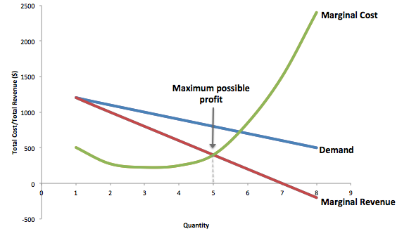
Table 2 expands Table 1 using the figures on total costs and total revenues from the HealthPill example to calculate marginal revenue and marginal cost. Recall that marginal revenue is the additional revenue the firm receives from selling one more (or a few more) units of output. Similarly, marginal cost is the additional cost the firm incurs from producing and selling one more (or a few more) units of output. This monopoly faces a typical U-shaped average cost curve and upward-sloping marginal cost curve, as shown in Figure 3.
| Quantity Q | Total Revenue TR | Marginal Revenue MR | Total Cost TC | Marginal Cost MC |
|---|---|---|---|---|
| 1 | 1,200 | 1,200 | 500 | 500 |
| 2 | 2,200 | 1,000 | 775 | 275 |
| 3 | 3,000 | 800 | 1,000 | 225 |
| 4 | 3,600 | 600 | 1,250 | 250 |
| 5 | 4,000 | 400 | 1,650 | 400 |
| 6 | 4,200 | 200 | 2,500 | 850 |
| 7 | 4,200 | 0 | 4,000 | 1,500 |
| 8 | 4,000 | –200 | 6,400 | 2,400 |
Notice that marginal revenue is zero at a quantity of 7, and turns negative at quantities higher than 7. It may seem counterintuitive that marginal revenue could ever be zero or negative: after all, doesn’t an increase in quantity sold always mean more revenue? For a perfect competitor, each additional unit sold brought a positive marginal revenue, because marginal revenue was equal to the given market price. However, a monopolist can sell a larger quantity and see a decline in total revenue, since in order to sell more output, the monopolist must cut the price. As the quantity sold becomes higher, at some point the drop in price is proportionally more than the increase in greater quantity of sales, causing a situation where more sales bring in less revenue. In other words, marginal revenue is negative.
A monopolist can determine its profit-maximizing price and quantity by analyzing the marginal revenue and marginal costs of producing an extra unit. If the marginal revenue exceeds the marginal cost, then the firm can increase profit by producing one more unit of output.
For example, at an output of 4 in Figure 3, marginal revenue is 600 and marginal cost is 250, so producing this unit will clearly add to overall profits. At an output of 5, marginal revenue is 400 and marginal cost is 400, so producing this unit still means overall profits are unchanged. However, expanding output from 5 to 6 would involve a marginal revenue of 200 and a marginal cost of 850, so that sixth unit would actually reduce profits. Thus, the monopoly can tell from the marginal revenue and marginal cost that of the choices in the table, the profit-maximizing level of output is 5.
The monopoly could seek out the profit-maximizing level of output by increasing quantity by a small amount, calculating marginal revenue and marginal cost, and then either increasing output as long as marginal revenue exceeds marginal cost or reducing output if marginal cost exceeds marginal revenue. This process works without any need to calculate total revenue and total cost. Thus, a profit-maximizing monopoly should follow the rule of producing up to the quantity where marginal revenue is equal to marginal cost—that is, MR = MC. This quantity is easy to identify graphically, where MR and MC intersect.
Maximizing Profits
If you find it counterintuitive that producing where marginal revenue equals marginal cost will maximize profits, working through the numbers will help.
Step 1. Remember, we define marginal cost as the change in total cost from producing a small amount of additional output.
Step 2. Note that in Table 2, as output increases from 1 to 2 units, total cost increases from $500 to $775. As a result, the marginal cost of the second unit will be:
Step 3. Remember that, similarly, marginal revenue is the change in total revenue from selling a small amount of additional output.
Step 4. Note that in Table 2, as output increases from 1 to 2 units, total revenue increases from $1200 to $2200. As a result, the marginal revenue of the second unit will be:
Table 3 below repeats the marginal cost and marginal revenue data from Table 2, and adds two more columns. Marginal profit is the profitability of each additional unit sold. We define it as marginal revenue minus marginal cost. Finally, total profit is the sum of marginal profits. As long as marginal profit is positive, producing more output will increase total profits. When marginal profit turns negative, producing more output will decrease total profits. Total profit is maximized where marginal revenue equals marginal cost. In this example, maximum profit occurs at 5 units of output.
| Quantity Q | Marginal Revenue MR | Marginal Cost MC | Marginal Profit MP | Total Profit P |
|---|---|---|---|---|
| 1 | 1,200 | 500 | 700 | 700 |
| 2 | 1,000 | 275 | 725 | 1,425 |
| 3 | 800 | 225 | 575 | 2,000 |
| 4 | 600 | 250 | 350 | 2,350 |
| 5 | 400 | 400 | 0 | 2,350 |
| 6 | 200 | 850 | −650 | 1,700 |
| 7 | 0 | 1,500 | −1,500 | 200 |
| 8 | −200 | 2,400 | −2,600 | −2,400 |
A perfectly competitive firm will also find its profit-maximizing level of output where MR = MC. The key difference with a perfectly competitive firm is that in the case of perfect competition, marginal revenue is equal to price (MR = P), while for a monopolist, marginal revenue is not equal to the price, because changes in quantity of output affect the price.
Choosing the Price
Once the monopolist identifies the profit maximizing quantity of output, the next step is to determine the corresponding price. This is straightforward if you remember that a firm’s demand curve shows the maximum price a firm can charge to sell any quantity of output. Graphically, start from the profit maximizing quantity in Figure 3, which is 5 units of output. Draw a vertical line up to the demand curve. Then read the price off the demand curve (i.e. $800).
Watch It
Watch the clip to review how a monopolist maximizes price and to see it on a graph.
An interactive or media element has been excluded from this version of the text. You can view it online here: http://pb.libretexts.org/mecon/?p=366
Why is a monopolist’s marginal revenue always less than the price?
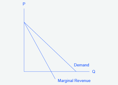
The marginal revenue curve for a monopolist always lies beneath the market demand curve. To understand why, think about increasing the quantity along the demand curve by one unit, so that you take one step down the demand curve to a slightly higher quantity but a slightly lower price. A demand curve is not sequential: it is not that first we sell Q1 at a higher price, and then we sell Q2 at a lower price. Rather, a demand curve is conditional: if we charge the higher price, we would sell Q1. If, instead, we charge a lower price (on all the units that we sell), we would sell Q2.
So when we think about increasing the quantity sold by one unit, marginal revenue is affected in two ways. First, we sell one additional unit at the new market price. Second, all the previous units, which could have been sold at the higher price, now sell for less. Because of the lower price on all units sold, the marginal revenue of selling a unit is less than the price of that unit—and the marginal revenue curve is below the demand curve.
Tip: For a straight-line demand curve, the marginal revenue curve equals price at the lowest level of output. (Graphically, MR and demand have the same vertical axis.) As output increases, marginal revenue decreases twice as fast as demand, so that the horizontal intercept of MR is halfway to the horizontal intercept of demand. You can see this in the Figure 4.
Glossary
[glossary-page][glossary-term]marginal profit: [/glossary-term]
[glossary-definition]profit of one more unit of output, computed as marginal revenue minus marginal cost[/glossary-definition][/glossary-page]
- Modification, adaptation, and original content. Provided by: Lumen Learning. License: CC BY: Attribution
- How a Profit-Maximizing Monopoly Chooses Output and Price. Authored by: OpenStax College. Located at: https://cnx.org/contents/vEmOH-_p@4.40:nZyOdEt7@4/How-a-Profit-Maximizing-Monopo#Table_09_03. License: CC BY: Attribution. License Terms: Download for free at http://cnx.org/contents/bc498e1f-efe...569ad09a82@4.4
- Maximizing Profit Under Monopoly. Provided by: Marginal Revolution University. Located at: https://www.youtube.com/watch?time_continue=209&v=IEjcTLPtTIY. License: Other. License Terms: Standard YouTube License