9.15: The Production Function
- Page ID
- 48395
\( \newcommand{\vecs}[1]{\overset { \scriptstyle \rightharpoonup} {\mathbf{#1}} } \)
\( \newcommand{\vecd}[1]{\overset{-\!-\!\rightharpoonup}{\vphantom{a}\smash {#1}}} \)
\( \newcommand{\id}{\mathrm{id}}\) \( \newcommand{\Span}{\mathrm{span}}\)
( \newcommand{\kernel}{\mathrm{null}\,}\) \( \newcommand{\range}{\mathrm{range}\,}\)
\( \newcommand{\RealPart}{\mathrm{Re}}\) \( \newcommand{\ImaginaryPart}{\mathrm{Im}}\)
\( \newcommand{\Argument}{\mathrm{Arg}}\) \( \newcommand{\norm}[1]{\| #1 \|}\)
\( \newcommand{\inner}[2]{\langle #1, #2 \rangle}\)
\( \newcommand{\Span}{\mathrm{span}}\)
\( \newcommand{\id}{\mathrm{id}}\)
\( \newcommand{\Span}{\mathrm{span}}\)
\( \newcommand{\kernel}{\mathrm{null}\,}\)
\( \newcommand{\range}{\mathrm{range}\,}\)
\( \newcommand{\RealPart}{\mathrm{Re}}\)
\( \newcommand{\ImaginaryPart}{\mathrm{Im}}\)
\( \newcommand{\Argument}{\mathrm{Arg}}\)
\( \newcommand{\norm}[1]{\| #1 \|}\)
\( \newcommand{\inner}[2]{\langle #1, #2 \rangle}\)
\( \newcommand{\Span}{\mathrm{span}}\) \( \newcommand{\AA}{\unicode[.8,0]{x212B}}\)
\( \newcommand{\vectorA}[1]{\vec{#1}} % arrow\)
\( \newcommand{\vectorAt}[1]{\vec{\text{#1}}} % arrow\)
\( \newcommand{\vectorB}[1]{\overset { \scriptstyle \rightharpoonup} {\mathbf{#1}} } \)
\( \newcommand{\vectorC}[1]{\textbf{#1}} \)
\( \newcommand{\vectorD}[1]{\overrightarrow{#1}} \)
\( \newcommand{\vectorDt}[1]{\overrightarrow{\text{#1}}} \)
\( \newcommand{\vectE}[1]{\overset{-\!-\!\rightharpoonup}{\vphantom{a}\smash{\mathbf {#1}}}} \)
\( \newcommand{\vecs}[1]{\overset { \scriptstyle \rightharpoonup} {\mathbf{#1}} } \)
\( \newcommand{\vecd}[1]{\overset{-\!-\!\rightharpoonup}{\vphantom{a}\smash {#1}}} \)
\(\newcommand{\avec}{\mathbf a}\) \(\newcommand{\bvec}{\mathbf b}\) \(\newcommand{\cvec}{\mathbf c}\) \(\newcommand{\dvec}{\mathbf d}\) \(\newcommand{\dtil}{\widetilde{\mathbf d}}\) \(\newcommand{\evec}{\mathbf e}\) \(\newcommand{\fvec}{\mathbf f}\) \(\newcommand{\nvec}{\mathbf n}\) \(\newcommand{\pvec}{\mathbf p}\) \(\newcommand{\qvec}{\mathbf q}\) \(\newcommand{\svec}{\mathbf s}\) \(\newcommand{\tvec}{\mathbf t}\) \(\newcommand{\uvec}{\mathbf u}\) \(\newcommand{\vvec}{\mathbf v}\) \(\newcommand{\wvec}{\mathbf w}\) \(\newcommand{\xvec}{\mathbf x}\) \(\newcommand{\yvec}{\mathbf y}\) \(\newcommand{\zvec}{\mathbf z}\) \(\newcommand{\rvec}{\mathbf r}\) \(\newcommand{\mvec}{\mathbf m}\) \(\newcommand{\zerovec}{\mathbf 0}\) \(\newcommand{\onevec}{\mathbf 1}\) \(\newcommand{\real}{\mathbb R}\) \(\newcommand{\twovec}[2]{\left[\begin{array}{r}#1 \\ #2 \end{array}\right]}\) \(\newcommand{\ctwovec}[2]{\left[\begin{array}{c}#1 \\ #2 \end{array}\right]}\) \(\newcommand{\threevec}[3]{\left[\begin{array}{r}#1 \\ #2 \\ #3 \end{array}\right]}\) \(\newcommand{\cthreevec}[3]{\left[\begin{array}{c}#1 \\ #2 \\ #3 \end{array}\right]}\) \(\newcommand{\fourvec}[4]{\left[\begin{array}{r}#1 \\ #2 \\ #3 \\ #4 \end{array}\right]}\) \(\newcommand{\cfourvec}[4]{\left[\begin{array}{c}#1 \\ #2 \\ #3 \\ #4 \end{array}\right]}\) \(\newcommand{\fivevec}[5]{\left[\begin{array}{r}#1 \\ #2 \\ #3 \\ #4 \\ #5 \\ \end{array}\right]}\) \(\newcommand{\cfivevec}[5]{\left[\begin{array}{c}#1 \\ #2 \\ #3 \\ #4 \\ #5 \\ \end{array}\right]}\) \(\newcommand{\mattwo}[4]{\left[\begin{array}{rr}#1 \amp #2 \\ #3 \amp #4 \\ \end{array}\right]}\) \(\newcommand{\laspan}[1]{\text{Span}\{#1\}}\) \(\newcommand{\bcal}{\cal B}\) \(\newcommand{\ccal}{\cal C}\) \(\newcommand{\scal}{\cal S}\) \(\newcommand{\wcal}{\cal W}\) \(\newcommand{\ecal}{\cal E}\) \(\newcommand{\coords}[2]{\left\{#1\right\}_{#2}}\) \(\newcommand{\gray}[1]{\color{gray}{#1}}\) \(\newcommand{\lgray}[1]{\color{lightgray}{#1}}\) \(\newcommand{\rank}{\operatorname{rank}}\) \(\newcommand{\row}{\text{Row}}\) \(\newcommand{\col}{\text{Col}}\) \(\renewcommand{\row}{\text{Row}}\) \(\newcommand{\nul}{\text{Nul}}\) \(\newcommand{\var}{\text{Var}}\) \(\newcommand{\corr}{\text{corr}}\) \(\newcommand{\len}[1]{\left|#1\right|}\) \(\newcommand{\bbar}{\overline{\bvec}}\) \(\newcommand{\bhat}{\widehat{\bvec}}\) \(\newcommand{\bperp}{\bvec^\perp}\) \(\newcommand{\xhat}{\widehat{\xvec}}\) \(\newcommand{\vhat}{\widehat{\vvec}}\) \(\newcommand{\uhat}{\widehat{\uvec}}\) \(\newcommand{\what}{\widehat{\wvec}}\) \(\newcommand{\Sighat}{\widehat{\Sigma}}\) \(\newcommand{\lt}{<}\) \(\newcommand{\gt}{>}\) \(\newcommand{\amp}{&}\) \(\definecolor{fillinmathshade}{gray}{0.9}\)Learning Objectives
- Explain the concept of a production function
- Differentiate between fixed and variable inputs
- Differentiate between total and marginal product
- Describe diminishing marginal productivity
We can summarize the ideas so far in terms of a production function, a mathematical expression or equation that explains the relationship between a firm’s inputs and its outputs:
A production is purely an engineering concept. If you plug in the amount of labor, capital and other inputs the firm is using, the production function tells how much output will be produced by those inputs. Production functions are specific to the product. Different products have different production functions. The amount of labor a farmer uses to produce a bushel of corn is likely different than that required to produce an automobile. Firms in the same industry may have somewhat different production functions, since each firm may produce a little differently. One pizza restaurant may make its own dough and sauce, while another may buy those pre-made. A sit-down pizza restaurant probably uses more labor (to handle table service) than a purely take-out restaurant. We can describe inputs as either fixed or variable.
Fixed inputs are those that can’t easily be increased or decreased in a short period of time. In the pizza example, the building is a fixed input. Once the entrepreneur signs the lease, he or she is stuck in the building until the lease expires. Fixed inputs define the firm’s maximum output capacity. This is analogous to the potential real GDP shown by society’s production possibilities curve, i.e. the maximum quantities of outputs a society can produce at a given time with its available resources. Fixed inputs do not change as output changes.
Variable inputs are those that can easily be increased or decreased in a short period of time. The pizzaiolo can order more ingredients with a phone call, so ingredients would be variable inputs. The owner could hire a new person to work the counter pretty quickly as well. Variable inputs increase or decrease as output changes.
Economists often use a short-hand form for the production function:
where L represents all the variable inputs, and K represents all the fixed inputs.
Economists also differentiate between short and long run production. The short run is the period of time during which at least some factors of production are fixed. During the period of the pizza restaurant lease, the pizza restaurant is operating in the short run, because it is limited to using the current building—the owner can’t choose a larger or smaller building. The long run is the period of time during which all factors are variable. Once the lease expires for the pizza restaurant, the shop owner can move to a larger or smaller place.
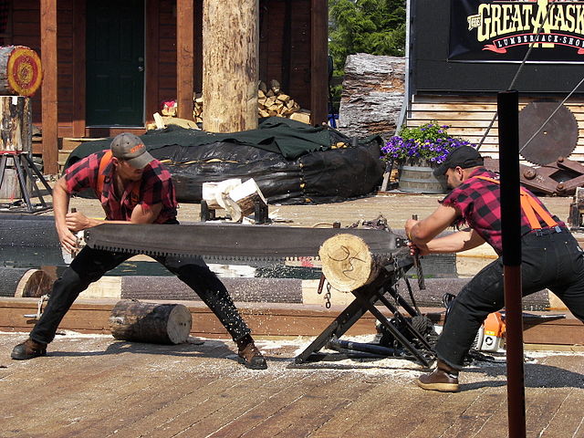
Note that there is another important distinction between fixed and variable inputs. In the short run, since the firm’s fixed inputs are fixed, the only way to vary a firm’s output is by changing its variable inputs. Let’s explore production in the short run using a specific example: tree cutting (for lumber) with a two-person crosscut saw.

Since by definition capital is fixed in the short run, our production function becomes
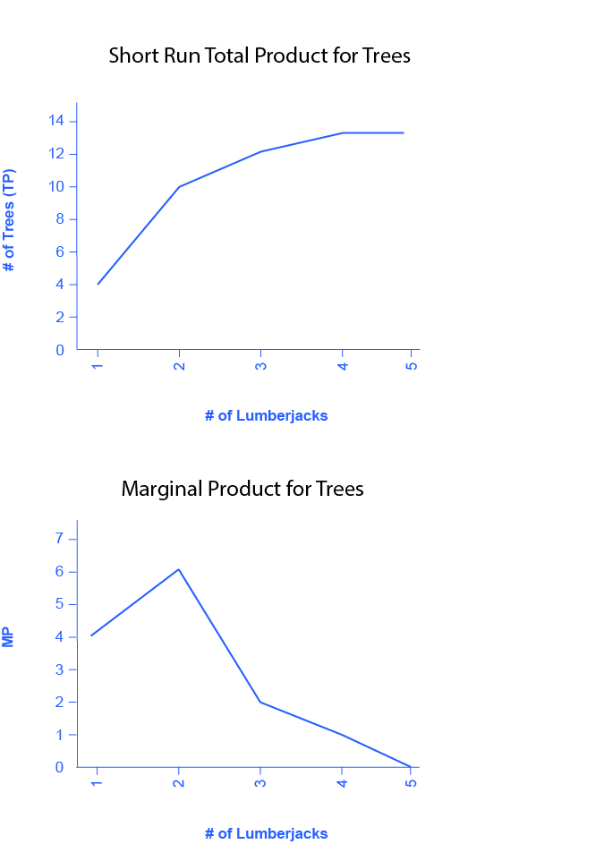
This equation simply indicates that since capital is fixed, then changing the amount of output (e.g. trees cut down per day) depends only on changing the amount of labor employed (e.g. number of lumberjacks working). We can express this production function numerically as Table 1 below shows. You can also see it graphically in Figure 2a.
| # Lumberjacks | 1 | 2 | 3 | 4 | 5 |
| # Trees (TP) | 4 | 10 | 12 | 13 | 13 |
| MP | 4 | 6 | 2 | 1 | 0 |

Note that we have introduced some new language. We also call Output (Q) Total Product (TP), which means the amount of output produced with a given amount of labor and a fixed amount of capital. In this example, one lumberjack using a two-person saw can cut down four trees in an hour. Two lumberjacks using a two-person saw can cut down ten trees in an hour.
We should also introduce a critical concept: marginal product. Marginal product is the additional output of one more worker. Mathematically, Marginal Product is the change in total product divided by the change in labor: In the table above, since 0 workers produce 0 trees, the marginal product of the first worker is four trees per day, but the marginal product of the second worker is six trees per day. Why might that be the case? It’s because of the nature of the capital the workers are using. A two-person saw works much better with two persons than with one. Suppose we add a third lumberjack to the story. What will that person’s marginal product be? What will that person contribute to the team? Perhaps he or she can oil the saw’s teeth to keep it sawing smoothly or he or she could bring water to the two people sawing.
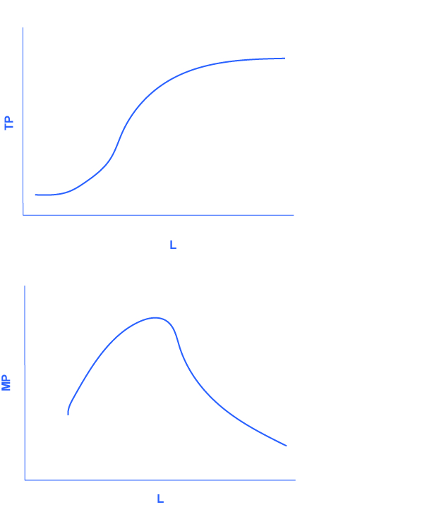
What you see in the table is a critically important conclusion about production in the short run: it may be that as we add workers, the marginal product increases at first, but sooner or later additional workers will have decreasing marginal product. In fact, there may eventually be no effect or a negative effect on output. This is called the Law of Diminishing Marginal Product and it’s a characteristic of production in the short run. Diminishing marginal productivity is very similar to the concept of diminishing marginal utility that we learned about in the chapter on consumer choice. Both concepts are examples of the more general concept of diminishing marginal returns. Why does diminishing marginal productivity occur? It’s because of fixed capital. We will see this more clearly when we discuss production in the long run.
We can show these concepts graphically, as you can see in Figure 2 above. Figure 3 shows the more general cases of total product and marginal product curves.

Try It
https://assessments.lumenlearning.co...sessments/7981
https://assessments.lumenlearning.co...sessments/7982
Watch It
Watch this video to review all of the production function and to see an example of the law of diminishing marginal product. Dr. McGlasson wants to hire students for her company to make “I love economics” signs, but she must consider how much output she can gain with each additional employee.
Try It
These questions allow you to get as much practice as you need, as you can click the link at the top of the first question (“Try another version of these questions”) to get a new set of questions. Practice until you feel comfortable doing the questions.
[ohm_question]154922-154927[/ohm_question]
Learning Objectives
- [glossary-page][glossary-term]factors of production (or inputs):[/glossary-term]
[glossary-definition]resources that firms use to produce their products, for example, labor and capital[/glossary-definition][glossary-term]firm:[/glossary-term]
[glossary-definition]an organization that combines inputs of labor, capital, land, and raw or finished component materials to produce outputs.[/glossary-definition][glossary-term]fixed inputs:[/glossary-term]
[glossary-definition]factors of production that can’t be easily increased or decreased in a short period of time[/glossary-definition][glossary-term]long run: [/glossary-term]
[glossary-definition]period of time during which all of the firm’s inputs are variable[/glossary-definition][glossary-term]production:[/glossary-term]
[glossary-definition]the process of combining inputs to produce outputs, ideally of a value greater than the value of the inputs[/glossary-definition][glossary-term]production function:[/glossary-term]
[glossary-definition]mathematical equation that tells how much output a firm can produce with given amounts of inputs[/glossary-definition][glossary-term]short run:[/glossary-term]
[glossary-definition]period of time during which at least one or more of the firm’s inputs is fixed[/glossary-definition][glossary-term]variable inputs:[/glossary-term]
[glossary-definition]factors of production that a firm can easily increase or decrease in a short period of time[/glossary-definition]
[/glossary-page]
Contributors and Attributions
- Modification, adaptation, and original content. Provided by: Lumen Learning. License: CC BY: Attribution
- Production in the Short Run. Provided by: OpenStax College. Located at: https://cnx.org/contents/XAl2LLVA@7.23:mS_p15F-@11/Production-in-the-Short-Run. License: CC BY: Attribution
- Episode 20: Producer Theory. Authored by: Dr. Mary McGlasson. Located at: https://www.youtube.com/watch?v=rnEFtyMzjOo. License: CC BY-NC-ND: Attribution-NonCommercial-NoDerivatives

