8.15: Income Changes and Consumption Choices
- Page ID
- 48383
Learning Objectives
- Demonstrate how changes in income and price affect consumer choices
- Contrast the substitution effect and the income effect
Consumer equilibrium, that is, the combination of goods and services that will maximize a consumer’s utility, depends on the consumers tastes and preferences, as expressed by his or her marginal utility numbers, the prices of those items and and the budget (or income) the consumer has. In this section, we will explore how changes in a consumer’s income and changes in the prices of goods and services affect consumer choice. Then, because the budget constraint framework can be used to analyze how quantities demanded change because of price movements, the budget constraint model can illustrate the underlying logic behind demand curves.
How Changes in Income Affect Consumer Choices
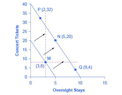
Let’s begin with a concrete example illustrating how changes in income level affect consumer choices. Figure 1 shows a budget constraint that represents Jazmin’s choice between concert tickets at $50 each and getting away overnight to a bed-and-breakfast for $200 per night. Jazmin has $1,000 per year to spend between these two choices. Jazmin could spend all of her budget on concert tickets, in which case she could buy $1000/$50 = 20 concert tickets. This shows the vertical axis of the budget constraint (zero B&B nights and 20 concert tickets). Alternatively, she could spent all of her budget on nights at a bed-and-breakfast, in which case she could afford $1000/200 = 5 nights. This shows the horizontal axis of her budget constraint (5 B&B nights and zero concert tickets.
After thinking about her total utility and marginal utility and applying the decision rules for maximizing utility explained earlier, Jazmin chooses point M, with eight concerts and three overnight getaways as her utility-maximizing choice.

Now, assume that the income Jazmin has to spend on these two items rises to $2,000 per year. Since the prices of the two products haven’t changed, doubling her budget allows Jazmin to purchase twice as many of each. This can be shown as a rightward shift in the budget constraint with intercepts as (0, 40) and (10, 0). How does this rise in income alter her utility-maximizing choice? Jazmin will again consider the total utility and marginal utility that she receives from concert tickets and overnight getaways to identify the consumer equilibrium on the new budget line. But how will her new choice relate to her original choice?
The possible choices along the new budget constraint can be divided into three groups, which are divided up by the dashed horizontal and vertical lines that pass through the original choice M in the figure. All choices on the upper left of the new budget constraint that are to the left of the vertical dashed line, like choice P with two overnight stays and 32 concert tickets, involve less of the good on the horizontal axis but much more of the good on the vertical axis. All choices to the right of the vertical dashed line and above the horizontal dashed line—like choice N with five overnight getaways and 20 concert tickets—have more consumption of both goods. Finally, all choices that are to the right of the vertical dashed line but below the horizontal dashed line, like choice Q with four concerts and nine overnight getaways, involve less of the good on the vertical axis but much more of the good on the horizontal axis.
All of these choices are theoretically possible, depending on Jazmin’s personal preferences as expressed through the total and marginal utility she would receive from consuming these two goods. When income rises, the most common reaction is to purchase more of both goods, like choice N, which is to the upper right relative to Jazmin’s original choice M, although exactly how much more of each good will vary according to personal taste. Conversely, when income falls, the most typical reaction is to purchase less of both goods. As we learned already in the module on elasticity, goods and services are called normal goods if a rise in income leads to a rise in the quantity consumed of that good and a fall in income leads to a fall in quantity consumed.
However, depending on Jazmin’s preferences, a rise in income could cause consumption of one good to increase while consumption of the other good declines. A choice like P means that a rise in income caused her quantity consumed of overnight stays to decline, while a choice like Q would mean that a rise in income caused her quantity of concerts to decline. Goods where demand declines as income rises (or conversely, where the demand rises as income falls) are called “inferior goods.” An inferior good occurs when people trim back on a good as income rises, because they can now afford the more expensive choices that they prefer. For example, a higher-income household might eat fewer hamburgers or be less likely to buy a used car, and instead eat more steak and buy a new car.
How Price Changes Affect Consumer Choices
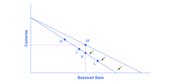
For analyzing the possible effect of a change in price on consumption, let’s again use a concrete example. Figure 2 represents the consumer choice of Sergei, who chooses between purchasing baseball bats and cameras. A price increase for baseball bats would have no effect on the ability to purchase cameras, but it would reduce the number of bats Sergei could afford to buy. Thus a price increase for baseball bats, the good on the horizontal axis, causes the budget constraint to rotate inward, as if on a hinge, from the vertical axis. As in the previous section, the point labeled M represents the originally preferred point on the original budget constraint, which Sergei has chosen after contemplating his total utility and marginal utility and the tradeoffs involved along the budget constraint. In this example, the units along the horizontal and vertical axes are not numbered, so the discussion must focus on whether more or less of certain goods will be consumed, not on numerical amounts.

After the price increase, Sergei will make a choice along the new budget constraint. Again, his choices can be divided into three segments by the dashed vertical and horizontal lines. In the upper left portion of the new budget constraint, at a choice like H, Sergei consumes more cameras and fewer bats. In the central portion of the new budget constraint, at a choice like J, he consumes less of both goods. At the right-hand end, at a choice like L, he consumes more bats but fewer cameras.
The typical response to higher prices is that a person chooses to consume less of the product with the higher price. This occurs for two reasons, and both effects can occur simultaneously. The substitution effect, which is more intuitive, occurs when the price of one good increases, giving consumers have an incentive to consume less of the good with the relatively higher price and more of the other good with a relatively lower price. In other words, the higher price of one good causes consumers to substitute the cheaper good for the more expensive one. The income effect, which is more subtle, notes that a higher price means, in effect, the buying power of one’s budget has been reduced (even though actual income has not changed), which leads to buying less of both goods (assuming both are normal goods).
In this example, the higher price for baseball bats would cause Sergei to buy fewer bats, both because of the substitution effect and because of the income effect. Exactly how much will a higher price for bats cause Sergei consumption of bats to fall? Figure 2 suggests a range of possibilities. Sergei might react to a higher price for baseball bats by purchasing the same quantity of bats, but cutting his consumption of cameras. This choice is the point K on the new budget constraint, straight below the original choice M. Alternatively, Sergei might react by dramatically reducing his purchases of bats and instead buy more cameras.
Note that the income effect also causes Sergei’s demand for cameras to fall, while the substitution effect increases demand. The net effect is not clear without specific measurements of the two effects. The key takeaway here is that it would be imprudent to assume that a change in the price of one good will only or primarily affect the good whose price is changed, while the quantity consumed of other goods remains the same. Since Sergei purchases all his products out of the same budget, a change in the price of one good can also have a range of effects, either positive or negative, on the quantity consumed of other goods. In short, a higher price typically causes reduced consumption of the good in question, but it can affect the consumption of other goods as well.
Watch It
We watched the first part of this video earlier when learning about budget constraints, and now we can watch the rest to see how the budget constraint graph changes with a change in budget or a change in the price of the goods.
An interactive or media element has been excluded from this version of the text. You can view it online here: http://pb.libretexts.org/mecon/?p=260
Try It
These questions allow you to get as much practice as you need, as you can click the link at the top of the first question (“Try another version of these questions”) to get a new set of questions. Practice until you feel comfortable doing the questions.
[ohm_question]155323-155324-155325[/ohm_question]
Glossary
[glossary-page][glossary-term]budget constraint:[/glossary-term]
[glossary-definition] all possible consumption combinations of goods that someone can afford, given the prices of goods, when all income is spent; the boundary of the opportunity set[/glossary-definition][glossary-term]income effect:[/glossary-term]
[glossary-definition] a higher price means that, in effect, the buying power of income has been reduced, even though actual income has not changed; always happens simultaneously with a substitution effect[/glossary-definition][glossary-term]substitution effect:[/glossary-term]
[glossary-definition] when a price changes, consumers have an incentive to consume less of the good with a relatively higher price and more of the good with a relatively low price[/glossary-definition]
[/glossary-page]
- Modification, adaptation, and original content. Provided by: Lumen Learning. License: CC BY: Attribution. License Terms: Download for free at http://cnx.org/contents/bc498e1f-efe...69ad09a82@4.44
- How Changes in Income and Prices Affect Consumption Choices. Authored by: OpenStax College. Located at: https://cnx.org/contents/vEmOH-_p@4.40:cCMVAG8i/How-Changes-in-Income-and-Pric. License: CC BY: Attribution. License Terms: Download for free at http://cnx.org/contents/bc498e1f-efe...569ad09a82@4.4
- Introduction to Consumer Choice. Provided by: Marginal Revolution University. Located at: https://www.youtube.com/watch?v=oG_R1jQPqTc. License: Other. License Terms: Standard YouTube License

