
8.10: Consumer Choice and Utility
- Page ID
- 48377
\( \newcommand{\vecs}[1]{\overset { \scriptstyle \rightharpoonup} {\mathbf{#1}} } \)
\( \newcommand{\vecd}[1]{\overset{-\!-\!\rightharpoonup}{\vphantom{a}\smash {#1}}} \)
\( \newcommand{\id}{\mathrm{id}}\) \( \newcommand{\Span}{\mathrm{span}}\)
( \newcommand{\kernel}{\mathrm{null}\,}\) \( \newcommand{\range}{\mathrm{range}\,}\)
\( \newcommand{\RealPart}{\mathrm{Re}}\) \( \newcommand{\ImaginaryPart}{\mathrm{Im}}\)
\( \newcommand{\Argument}{\mathrm{Arg}}\) \( \newcommand{\norm}[1]{\| #1 \|}\)
\( \newcommand{\inner}[2]{\langle #1, #2 \rangle}\)
\( \newcommand{\Span}{\mathrm{span}}\)
\( \newcommand{\id}{\mathrm{id}}\)
\( \newcommand{\Span}{\mathrm{span}}\)
\( \newcommand{\kernel}{\mathrm{null}\,}\)
\( \newcommand{\range}{\mathrm{range}\,}\)
\( \newcommand{\RealPart}{\mathrm{Re}}\)
\( \newcommand{\ImaginaryPart}{\mathrm{Im}}\)
\( \newcommand{\Argument}{\mathrm{Arg}}\)
\( \newcommand{\norm}[1]{\| #1 \|}\)
\( \newcommand{\inner}[2]{\langle #1, #2 \rangle}\)
\( \newcommand{\Span}{\mathrm{span}}\) \( \newcommand{\AA}{\unicode[.8,0]{x212B}}\)
\( \newcommand{\vectorA}[1]{\vec{#1}} % arrow\)
\( \newcommand{\vectorAt}[1]{\vec{\text{#1}}} % arrow\)
\( \newcommand{\vectorB}[1]{\overset { \scriptstyle \rightharpoonup} {\mathbf{#1}} } \)
\( \newcommand{\vectorC}[1]{\textbf{#1}} \)
\( \newcommand{\vectorD}[1]{\overrightarrow{#1}} \)
\( \newcommand{\vectorDt}[1]{\overrightarrow{\text{#1}}} \)
\( \newcommand{\vectE}[1]{\overset{-\!-\!\rightharpoonup}{\vphantom{a}\smash{\mathbf {#1}}}} \)
\( \newcommand{\vecs}[1]{\overset { \scriptstyle \rightharpoonup} {\mathbf{#1}} } \)
\( \newcommand{\vecd}[1]{\overset{-\!-\!\rightharpoonup}{\vphantom{a}\smash {#1}}} \)
\(\newcommand{\avec}{\mathbf a}\) \(\newcommand{\bvec}{\mathbf b}\) \(\newcommand{\cvec}{\mathbf c}\) \(\newcommand{\dvec}{\mathbf d}\) \(\newcommand{\dtil}{\widetilde{\mathbf d}}\) \(\newcommand{\evec}{\mathbf e}\) \(\newcommand{\fvec}{\mathbf f}\) \(\newcommand{\nvec}{\mathbf n}\) \(\newcommand{\pvec}{\mathbf p}\) \(\newcommand{\qvec}{\mathbf q}\) \(\newcommand{\svec}{\mathbf s}\) \(\newcommand{\tvec}{\mathbf t}\) \(\newcommand{\uvec}{\mathbf u}\) \(\newcommand{\vvec}{\mathbf v}\) \(\newcommand{\wvec}{\mathbf w}\) \(\newcommand{\xvec}{\mathbf x}\) \(\newcommand{\yvec}{\mathbf y}\) \(\newcommand{\zvec}{\mathbf z}\) \(\newcommand{\rvec}{\mathbf r}\) \(\newcommand{\mvec}{\mathbf m}\) \(\newcommand{\zerovec}{\mathbf 0}\) \(\newcommand{\onevec}{\mathbf 1}\) \(\newcommand{\real}{\mathbb R}\) \(\newcommand{\twovec}[2]{\left[\begin{array}{r}#1 \\ #2 \end{array}\right]}\) \(\newcommand{\ctwovec}[2]{\left[\begin{array}{c}#1 \\ #2 \end{array}\right]}\) \(\newcommand{\threevec}[3]{\left[\begin{array}{r}#1 \\ #2 \\ #3 \end{array}\right]}\) \(\newcommand{\cthreevec}[3]{\left[\begin{array}{c}#1 \\ #2 \\ #3 \end{array}\right]}\) \(\newcommand{\fourvec}[4]{\left[\begin{array}{r}#1 \\ #2 \\ #3 \\ #4 \end{array}\right]}\) \(\newcommand{\cfourvec}[4]{\left[\begin{array}{c}#1 \\ #2 \\ #3 \\ #4 \end{array}\right]}\) \(\newcommand{\fivevec}[5]{\left[\begin{array}{r}#1 \\ #2 \\ #3 \\ #4 \\ #5 \\ \end{array}\right]}\) \(\newcommand{\cfivevec}[5]{\left[\begin{array}{c}#1 \\ #2 \\ #3 \\ #4 \\ #5 \\ \end{array}\right]}\) \(\newcommand{\mattwo}[4]{\left[\begin{array}{rr}#1 \amp #2 \\ #3 \amp #4 \\ \end{array}\right]}\) \(\newcommand{\laspan}[1]{\text{Span}\{#1\}}\) \(\newcommand{\bcal}{\cal B}\) \(\newcommand{\ccal}{\cal C}\) \(\newcommand{\scal}{\cal S}\) \(\newcommand{\wcal}{\cal W}\) \(\newcommand{\ecal}{\cal E}\) \(\newcommand{\coords}[2]{\left\{#1\right\}_{#2}}\) \(\newcommand{\gray}[1]{\color{gray}{#1}}\) \(\newcommand{\lgray}[1]{\color{lightgray}{#1}}\) \(\newcommand{\rank}{\operatorname{rank}}\) \(\newcommand{\row}{\text{Row}}\) \(\newcommand{\col}{\text{Col}}\) \(\renewcommand{\row}{\text{Row}}\) \(\newcommand{\nul}{\text{Nul}}\) \(\newcommand{\var}{\text{Var}}\) \(\newcommand{\corr}{\text{corr}}\) \(\newcommand{\len}[1]{\left|#1\right|}\) \(\newcommand{\bbar}{\overline{\bvec}}\) \(\newcommand{\bhat}{\widehat{\bvec}}\) \(\newcommand{\bperp}{\bvec^\perp}\) \(\newcommand{\xhat}{\widehat{\xvec}}\) \(\newcommand{\vhat}{\widehat{\vvec}}\) \(\newcommand{\uhat}{\widehat{\uvec}}\) \(\newcommand{\what}{\widehat{\wvec}}\) \(\newcommand{\Sighat}{\widehat{\Sigma}}\) \(\newcommand{\lt}{<}\) \(\newcommand{\gt}{>}\) \(\newcommand{\amp}{&}\) \(\definecolor{fillinmathshade}{gray}{0.9}\)Learning Objectives
- Explain utility and its connection to consumer behavior
- Calculate the total utility of a collection of goods and services
Consumer Choices
Information on the consumption choices of Americans is available from the Consumer Expenditure Survey carried out by the U.S. Bureau of Labor Statistics. Figure 1 shows spending patterns for the average U.S. household. The first row shows income and, after taxes and personal savings are subtracted, it shows that, in 2015, the average U.S. household spent $48,109 on consumption. The table then breaks down consumption into various categories. The average U.S. household spent roughly one-third of its consumption on shelter and other housing expenses, another one-third on food and vehicle expenses, and the rest on a variety of items, as shown. These patterns will vary for specific households by differing levels of family income, by geography, and by preferences.
| Average Household Income before Taxes | $62,481 |
| Average Annual Expenditures | $48.109 |
| Food at home | $3,264 |
| Food away from home | $2,505 |
| Housing | $16,557 |
| Apparel and services | $1,700 |
| Transportation | $7,677 |
| Healthcare | $3,157 |
| Entertainment | $2,504 |
| Education | $1,074 |
| Personal insurance and pensions | $5,357 |
| All else: alcohol, tobacco, reading, personal care, cash contributions, miscellaneous | $3,356 |
When economists talk about consumer choice, what they are referring to is the combination of goods and services a consumer purchases. To understand how a household will make its choices, economists look at what consumers can afford, as shown in a budget constraint (or budget line), and the total utility or satisfaction derived from those choices. When we graph a budget constraint, the quantity of one good is on the horizontal axis and the quantity of the other good on the vertical axis. The budget constraint line shows the various combinations of two goods that are affordable given a specific budget (or level of consumer income).
Watch It
Watch the selected clip from this video to review budget constraints. The budget constraint graph shows the various combinations of goods (like coffee and pizza) that you can afford at any given price. We’ll finish the second portion of the video later in the module.
An interactive or media element has been excluded from this version of the text. You can view it online here: http://pb.libretexts.org/mecon/?p=250
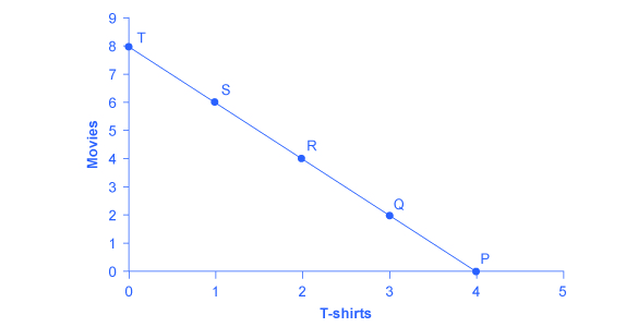
Consider José’s situation. José likes to collect T-shirts and watch movies. In Figure 1 we show the quantity of T-shirts on the horizontal axis while we show the quantity of movies on the vertical axis. If José had unlimited income or goods were free, then he could consume without limit. However, José, like all of us, faces a budget constraint. José has a total of $56 to spend. The price of T-shirts is $14 and the price of movies is $7. Notice that the vertical intercept of the budget constraint line is at eight movies and zero T-shirts ($56/$7=8). The horizontal intercept of the budget constraint is four, where José spends of all of his money on T-shirts and no movies ($56/14=4). The slope of the budget constraint line is rise/run or –8/4=–2. The specific choices along the budget constraint line show the combinations of affordable T-shirts and movies.
Utility is the term economists use to describe the satisfaction or happiness a person gets from consuming a good or service. José obtains utility from consuming T-shirts and consuming movies. Like all consumers, we assume José wishes to choose the combination of T-shirts and movies that will provide him with the greatest total utility,
Let’s begin with an assumption, which we will discuss in more detail later, that José can measure his own utility with something called utils. (It is important to note that you cannot make comparisons between the utils of individuals. If one person gets 20 utils from a cup of coffee and another gets 10 utils, this does not mean than the first person gets more enjoyment from the coffee than the other or that they enjoy the coffee twice as much. The reason why is that utils are subjective to an individual. The way one person measures utils is not the same as the way someone else does.)
| T-Shirts (Quantity) | Total Utility | Movies (Quantity) | Total Utility | ||
|---|---|---|---|---|---|
| 1 | 22 | 1 | 16 | ||
| 2 | 43 | 2 | 31 | ||
| 3 | 63 | 3 | 45 | ||
| 4 | 81 | 4 | 58 | ||
| 5 | 97 | 5 | 70 | ||
| 6 | 111 | 6 | 81 | ||
| 7 | 123 | 7 | 91 | ||
| 8 | 133 | 8 | 100 |
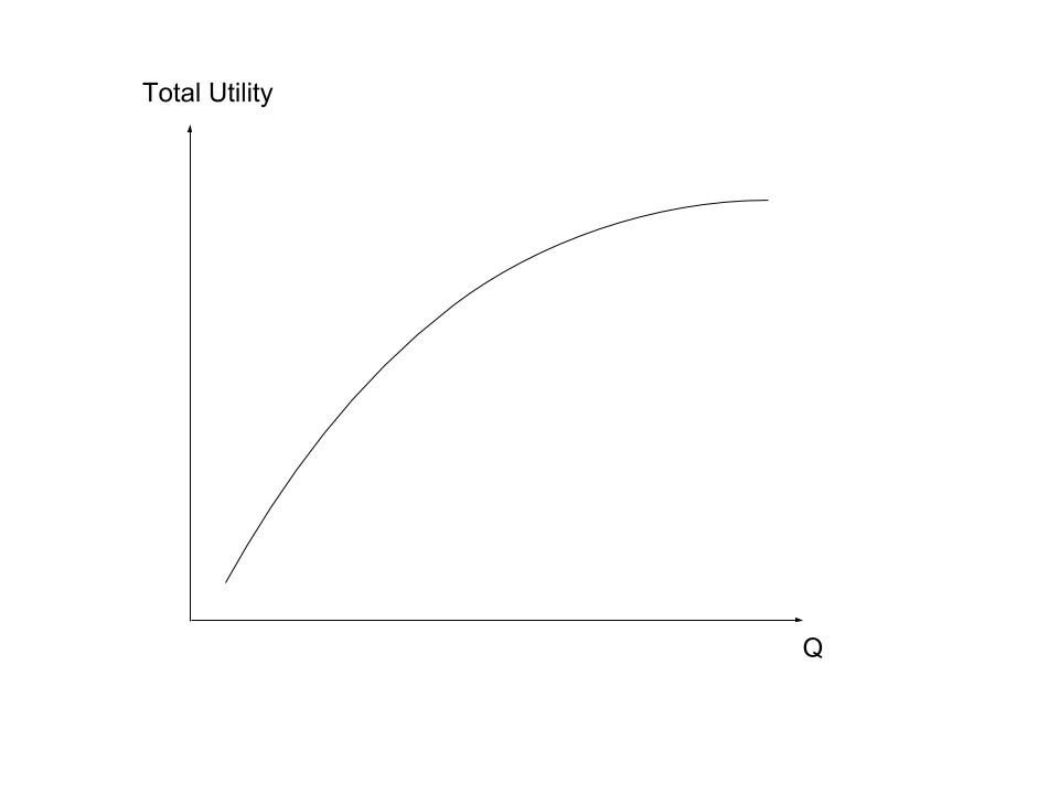
Table 2 shows how José’s utility is connected with his T-shirt or movie consumption. The first column of the table shows the quantity of T-shirts consumed. The second column shows the total utility, or total amount of satisfaction, that José receives from consuming that number of T-shirts. The typical pattern of total utility, shown in this example, is that consuming additional units of a good leads to greater total utility, but at a decreasing rate. We can see this in Figure 2.
The rest of Table 2 shows the utility José would obtain from attending different quantities of movies. Total utility follows the expected pattern: it increases as the number of movies that José watches rises. José can afford any combination of T-shirts and movies which is on his budget constraint. Which combination should he choose if he wishes to obtain the most utility possible? Table 3 looks at each point on the budget constraint in Figure 1, and adds up José’s total utility for each combination of T-shirts and movies.
| Point | T-Shirts | Movies | Total Utility |
|---|---|---|---|
| P | 4 | 0 | 81 + 0 = 81 |
| Q | 3 | 2 | 63 + 31 = 94 |
| R | 2 | 4 | 43 + 58 = 101 |
| S | 1 | 6 | 22 + 81 = 103 |
| T | 0 | 8 | 0 + 100 = 100 |
Calculating Total Utility
Let’s look at how José makes his decision in more detail.
Step 1. Observe that, at point Q in Figure 1 (for example), José consumes three T-shirts and two movies.
Step 2. Look at Table 2. You can see from the fourth row/second column that three T-shirts are worth 63 utils. Similarly, the second row/fifth column shows that two movies are worth 31 utils.
Step 3. From this information, you can calculate that point Q has a total utility of 94 (63 + 31).
Step 4. You can repeat the same calculations for each point on Table 3, in which the total utility numbers are shown in the last column.
For José, the highest total utility for all possible combinations of goods occurs at point S, with a total utility of 103 from consuming one T-shirt and six movies.
Try It
These questions allow you to get as much practice as you need, as you can click the link at the top of the first question (“Try another version of these questions”) to get a new set of questions. Practice until you feel comfortable doing the questions.
[ohm_question]155306-155307[/ohm_question]
Glossary
- [glossary-page][glossary-term]budget constraint (or budget line):[/glossary-term]
[glossary-definition]shows the possible combinations of two goods that are affordable given a consumer’s limited income[/glossary-definition][glossary-term]total utility:[/glossary-term]
[glossary-definition]the satisfaction a consumer gets from consuming some quantity of a good or service; also, it’s the total satisfaction from consuming all the goods and services an individual purchases.[/glossary-definition][glossary-term]utility:[/glossary-term]
[glossary-definition]the term economists use to describe the satisfaction or happiness a person gets from consuming a good or service.[/glossary-definition]
[/glossary-page]
- Consumption Choices. Authored by: OpenStax College. Located at: https://cnx.org/contents/vEmOH-_p@4.48:C_ifxn91@6/Consumption-Choices. License: CC BY: Attribution. License Terms: Download for free at http://cnx.org/contents/bc498e1f-efe...69ad09a82@4.44
- Budget Constraints. Provided by: Marginal Revolution University. Located at: https://www.youtube.com/watch?v=sNRZE0kwNGI. License: Other. License Terms: Standard YouTube License