3.4: Interpreting Slope

Last updated
Save as PDF

Page ID: 48294

$ \newcommand{\vecs}[1]{\overset { \scriptstyle \rightharpoonup} {\mathbf{#1}} } $

$ \newcommand{\vecd}[1]{\overset{-\!-\!\rightharpoonup}{\vphantom{a}\smash {#1}}} $

$ \newcommand{\id}{\mathrm{id}}$ $ \newcommand{\Span}{\mathrm{span}}$

( \newcommand{\kernel}{\mathrm{null}\,}\) $ \newcommand{\range}{\mathrm{range}\,}$

$ \newcommand{\RealPart}{\mathrm{Re}}$ $ \newcommand{\ImaginaryPart}{\mathrm{Im}}$

$ \newcommand{\Argument}{\mathrm{Arg}}$ $ \newcommand{\norm}[1]{\| #1 \|}$

$ \newcommand{\inner}[2]{\langle #1, #2 \rangle}$

$ \newcommand{\Span}{\mathrm{span}}$

$ \newcommand{\id}{\mathrm{id}}$

$ \newcommand{\Span}{\mathrm{span}}$

$ \newcommand{\kernel}{\mathrm{null}\,}$

$ \newcommand{\range}{\mathrm{range}\,}$

$ \newcommand{\RealPart}{\mathrm{Re}}$

$ \newcommand{\ImaginaryPart}{\mathrm{Im}}$

$ \newcommand{\Argument}{\mathrm{Arg}}$

$ \newcommand{\norm}[1]{\| #1 \|}$

$ \newcommand{\inner}[2]{\langle #1, #2 \rangle}$

$ \newcommand{\Span}{\mathrm{span}}$ $ \newcommand{\AA}{\unicode[.8,0]{x212B}}$

$ \newcommand{\vectorA}[1]{\vec{#1}} % arrow$

$ \newcommand{\vectorAt}[1]{\vec{\text{#1}}} % arrow$

$ \newcommand{\vectorB}[1]{\overset { \scriptstyle \rightharpoonup} {\mathbf{#1}} } $

$ \newcommand{\vectorC}[1]{\textbf{#1}} $

$ \newcommand{\vectorD}[1]{\overrightarrow{#1}} $

$ \newcommand{\vectorDt}[1]{\overrightarrow{\text{#1}}} $

$ \newcommand{\vectE}[1]{\overset{-\!-\!\rightharpoonup}{\vphantom{a}\smash{\mathbf {#1}}}} $

$ \newcommand{\vecs}[1]{\overset { \scriptstyle \rightharpoonup} {\mathbf{#1}} } $

$ \newcommand{\vecd}[1]{\overset{-\!-\!\rightharpoonup}{\vphantom{a}\smash {#1}}} $

$\newcommand{\avec}{\mathbf a}$ $\newcommand{\bvec}{\mathbf b}$ $\newcommand{\cvec}{\mathbf c}$ $\newcommand{\dvec}{\mathbf d}$ $\newcommand{\dtil}{\widetilde{\mathbf d}}$ $\newcommand{\evec}{\mathbf e}$ $\newcommand{\fvec}{\mathbf f}$ $\newcommand{\nvec}{\mathbf n}$ $\newcommand{\pvec}{\mathbf p}$ $\newcommand{\qvec}{\mathbf q}$ $\newcommand{\svec}{\mathbf s}$ $\newcommand{\tvec}{\mathbf t}$ $\newcommand{\uvec}{\mathbf u}$ $\newcommand{\vvec}{\mathbf v}$ $\newcommand{\wvec}{\mathbf w}$ $\newcommand{\xvec}{\mathbf x}$ $\newcommand{\yvec}{\mathbf y}$ $\newcommand{\zvec}{\mathbf z}$ $\newcommand{\rvec}{\mathbf r}$ $\newcommand{\mvec}{\mathbf m}$ $\newcommand{\zerovec}{\mathbf 0}$ $\newcommand{\onevec}{\mathbf 1}$ $\newcommand{\real}{\mathbb R}$ $\newcommand{\twovec}[2]{\left[\begin{array}{r}#1 \\ #2 \end{array}\right]}$ $\newcommand{\ctwovec}[2]{\left[\begin{array}{c}#1 \\ #2 \end{array}\right]}$ $\newcommand{\threevec}[3]{\left[\begin{array}{r}#1 \\ #2 \\ #3 \end{array}\right]}$ $\newcommand{\cthreevec}[3]{\left[\begin{array}{c}#1 \\ #2 \\ #3 \end{array}\right]}$ $\newcommand{\fourvec}[4]{\left[\begin{array}{r}#1 \\ #2 \\ #3 \\ #4 \end{array}\right]}$ $\newcommand{\cfourvec}[4]{\left[\begin{array}{c}#1 \\ #2 \\ #3 \\ #4 \end{array}\right]}$ $\newcommand{\fivevec}[5]{\left[\begin{array}{r}#1 \\ #2 \\ #3 \\ #4 \\ #5 \\ \end{array}\right]}$ $\newcommand{\cfivevec}[5]{\left[\begin{array}{c}#1 \\ #2 \\ #3 \\ #4 \\ #5 \\ \end{array}\right]}$ $\newcommand{\mattwo}[4]{\left[\begin{array}{rr}#1 \amp #2 \\ #3 \amp #4 \\ \end{array}\right]}$ $\newcommand{\laspan}[1]{\text{Span}\{#1\}}$ $\newcommand{\bcal}{\cal B}$ $\newcommand{\ccal}{\cal C}$ $\newcommand{\scal}{\cal S}$ $\newcommand{\wcal}{\cal W}$ $\newcommand{\ecal}{\cal E}$ $\newcommand{\coords}[2]{\left\{#1\right\}_{#2}}$ $\newcommand{\gray}[1]{\color{gray}{#1}}$ $\newcommand{\lgray}[1]{\color{lightgray}{#1}}$ $\newcommand{\rank}{\operatorname{rank}}$ $\newcommand{\row}{\text{Row}}$ $\newcommand{\col}{\text{Col}}$ $\renewcommand{\row}{\text{Row}}$ $\newcommand{\nul}{\text{Nul}}$ $\newcommand{\var}{\text{Var}}$ $\newcommand{\corr}{\text{corr}}$ $\newcommand{\len}[1]{\left|#1\right|}$ $\newcommand{\bbar}{\overline{\bvec}}$ $\newcommand{\bhat}{\widehat{\bvec}}$ $\newcommand{\bperp}{\bvec^\perp}$ $\newcommand{\xhat}{\widehat{\xvec}}$ $\newcommand{\vhat}{\widehat{\vvec}}$ $\newcommand{\uhat}{\widehat{\uvec}}$ $\newcommand{\what}{\widehat{\wvec}}$ $\newcommand{\Sighat}{\widehat{\Sigma}}$ $\newcommand{\lt}{<}$ $\newcommand{\gt}{>}$ $\newcommand{\amp}{&}$ $\definecolor{fillinmathshade}{gray}{0.9}$

Learning Objectives

Differentiate between a positive relationship and a negative relationship

Olympic skier tucked as he races downhill.

Figure 1. This skier speeds down the slope in an Olympic race. What’s your guess as to the steepness, or slope, of this ski hill?

What the Slope Means

The concept of slope is very useful in economics, because it measures the relationship between two variables. A positive slope means that two variables are positively related—that is, when x increases, so does y, and when x decreases, y also decreases. Graphically, a positive slope means that as a line on the line graph moves from left to right, the line rises. We will learn in other sections that “price” and “quantity supplied” have a positive relationship; that is, firms will supply more when the price is higher.

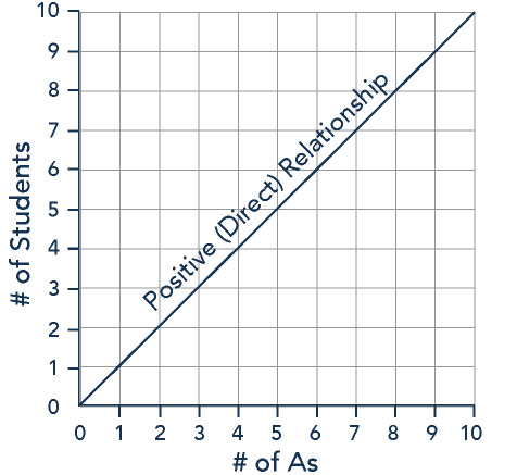
A graph with points (1,1) (2,2), and so on. As the x-axis (number of Fs) increases, so does the y-axis (number of students).

Figure 1. Positive Slope.

A negative slope means that two variables are negatively related; that is, when x increases, y decreases, and when x decreases, y increases. Graphically, a negative slope means that as the line on the line graph moves from left to right, the line falls. We will learn that “price” and “quantity demanded” have a negative relationship; that is, consumers will purchase less when the price is higher.

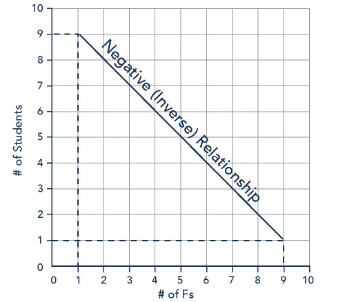
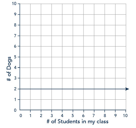
A graph with points (9,1) (8,2), and so on. As the x-axis (number of Fs) increases, the y-axis (number of students) decreases.

Figure 2. Negative slope.

A slope of zero means that y is constant no matter the value of x. Graphically, the line is flat; the rise over run is zero.

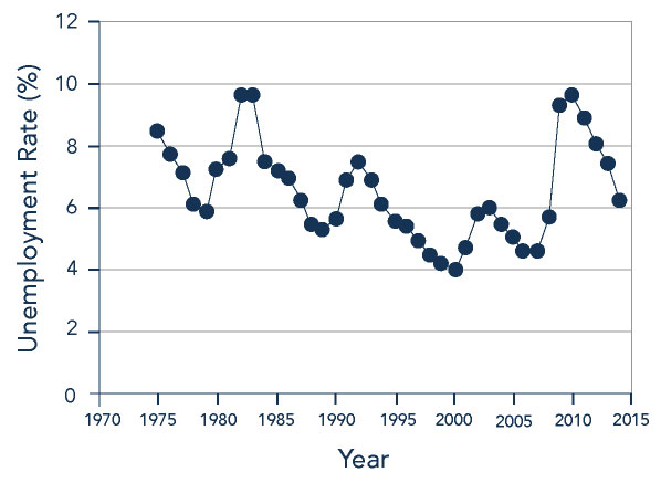
A graph with points (2,2), (3,2), (4,2) and so on. As the x-axis (number of students in the class) changes, the y-axis (the number of dogs) remains the same.

Figure 3. Slope of Zero

The unemployment-rate graph in Figure 4, below, illustrates a common pattern of many line graphs: some segments where the slope is positive, other segments where the slope is negative, and still other segments where the slope is close to zero.

The graph shows unemployment rates since 1970. The highest rates occurred around 1983 and 2010.

Figure 4. U.S. Unemployment Rate, 1975–2014.

Try It

https://assessments.lumenlearning.co...sessments/7082

Calculating Slope

The slope of a straight line between two points can be calculated in numerical terms. To calculate slope, begin by designating one point as the “starting point” and the other point as the “end point” and then calculating the rise over run between these two points.

Try It

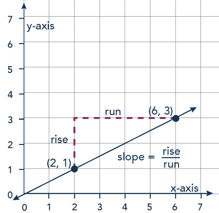
Use the graph to find the slope of the line.

A line that crosses the points (2,1) and (6,3). A blue line labeled Rise goes up two units from the point (2,1). A red line labeled Run goes left from the point (6,3) so that it forms a triangle with the main line and the Rise line. A formula says slope equals rise over run.

Figure 5.

[reveal-answer q=”246780″]Show Answer[/reveal-answer]
[hidden-answer a=”246780″]

Start from a point on the line, such as $(2,1)$ and move vertically until in line with another point on the line, such as $(6,3)$ . The rise is 2 units. It is positive as you moved up.

Next, move horizontally to the point $(6,3)$ . Count the number of units. The run is 4 units. It is positive as you moved to the right.

Then solve using the formula:

$\displaystyle \text{Slope }=\frac{\text{rise}}{\text{run}}$

$\displaystyle \text{Slope}=\frac{2}{4}=\frac{1}{2}$

Try It

These next questions allow you to get as much practice as you need, as you can click the link at the top of the first question (“Try another version of these questions”) to get a new set of questions. Practice until you feel comfortable doing the questions and then move on.

[ohm_question sameseed=1]92306-93504-92308[/ohm_question]

Graphs of economic relationships are not always straight lines. In this course, you will often see nonlinear (curved) lines, like Figure 6, which shows the relationship between quantity of output being produced and the cost of producing that output. As the quantity of output increases, the total cost increases at a faster rate. Table 1 shows the data behind this graph.

Table 1: Total Cost Curve
	Quantity of Output (Q)	Total Cost (TC)
	1	$1
	2	$4
	3	$9
“Point A”	4	$16
“Point B”	5	$25
	6	$36
	7	$49
	8	$64
	9	$81
	10	$100

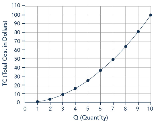
Graph showing total cost on the y-axis and quantity on the x-axis. The graph increases at a faster rate and slopes upward more rapidly towards the end. The graph moves through points (1,1) (2,4) (3,10) (4,18) (5,25) (6,38) (7,50) (8,65) (9, 85) (10, 100)

Figure 6. In this example, the total cost of production increase at a faster rate when the quantity of output increases.

We can interpret nonlinear relationships similarly to the way we interpret linear relationships. Their slopes can be positive or negative. We can calculate the slopes similarly also, looking at the rise over the run of a segment of a curve.

As an example, consider the slope of the total cost curve, above, between points A & B. Going from point A to point B, the rise is the change in total cost (i.e. the variable on the vertical axis):

$25 – $16 = $9

Similarly, the run is the change in quantity (i.e. the variable on the horizontal axis):

5 – 4 = 1

Thus, the slope of a straight line between these two points would be 9/1 = 9. In other words, as we increase the quantity of output produced by one unit, the total cost of production increases by $9.

Try It

https://assessments.lumenlearning.co...sessments/7083

Suppose the slope of a line were to increase. Graphically, that means it would get steeper. Suppose the slope of a line were to decrease. Then it would get flatter. These conditions are true whether or not the slope was positive or negative to begin with. A lower positive slope means a flatter upward tilt to the curve, which you can see in Figure 6 at low levels of output. A higher positive slope means a steeper upward tilt to the curve, which you can see at higher output levels.

A negative slope that is larger in absolute value (that is, more negative) means a steeper downward tilt to the line. A slope of zero is a horizontal line. A vertical line has an infinite slope.

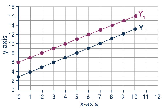
Suppose a line has a larger intercept. Graphically, that means it would shift out (or up) from the old origin, parallel to the old line. This is shown in Figure 7, below, as the shift from the line labeled Y to the line labeled Y₁. If a line has a smaller intercept, it would shift in (or down), parallel to the old line.

Graph showing a upward-sloping line going through points (0,3) (2,5) (3,6) (4,7), etc. that then moves outward and the entire line outward to (0,6) (1,7) (2,8) (3,9) (4,10)...

Figure 7. A larger y-intercept shifts the entire graph to cross the y-axis at a higher point.

Glossary

[glossary-page][glossary-term]negative slope: [/glossary-term]
[glossary-definition]indicates that two variables are negatively related; when one variable increases, the other decreases, and when one variable decreases, the other increases[/glossary-definition][glossary-term]positive slope:[/glossary-term][glossary-definition] indicates that two variables are positively related; when one variable increases, so does the other, and when one variable decreases, the other also decreases[/glossary-definition][glossary-term]slope: [/glossary-term]
[glossary-definition]the change in the vertical axis divided by the change in the horizontal axis[/glossary-definition][glossary-term]slope of zero: [/glossary-term][glossary-definition]indicates that there is no relationship between two variables; when one variable changes, the other does not change[/glossary-definition]
[/glossary-page]

Revision and adaptation. Provided by: Lumen Learning. License: CC BY: Attribution

Principles of Microeconomics Appendix. Authored by: OpenStax College. Provided by: Rice University. Located at: http://cnx.org/contents/6i8iXmBj@10.170:Nihva8h5@10/The-Use-of-Mathematics-in-Prin#CNX_Econ_A01_008. License: CC BY: Attribution. License Terms: Download for free at http://cnx.org/content/col11627/latest
Go Time. Authored by: Jon Wick. Located at: https://www.flickr.com/photos/jonwick/4369221975/. License: CC BY: Attribution

Search

Text Color

Text Size

Margin Size

Font Type

Learning Objectives

Try It

Try It

Try It

Try It

Glossary