
14.5: The Phillips Curve
- Page ID
- 47509
\( \newcommand{\vecs}[1]{\overset { \scriptstyle \rightharpoonup} {\mathbf{#1}} } \)
\( \newcommand{\vecd}[1]{\overset{-\!-\!\rightharpoonup}{\vphantom{a}\smash {#1}}} \)
\( \newcommand{\dsum}{\displaystyle\sum\limits} \)
\( \newcommand{\dint}{\displaystyle\int\limits} \)
\( \newcommand{\dlim}{\displaystyle\lim\limits} \)
\( \newcommand{\id}{\mathrm{id}}\) \( \newcommand{\Span}{\mathrm{span}}\)
( \newcommand{\kernel}{\mathrm{null}\,}\) \( \newcommand{\range}{\mathrm{range}\,}\)
\( \newcommand{\RealPart}{\mathrm{Re}}\) \( \newcommand{\ImaginaryPart}{\mathrm{Im}}\)
\( \newcommand{\Argument}{\mathrm{Arg}}\) \( \newcommand{\norm}[1]{\| #1 \|}\)
\( \newcommand{\inner}[2]{\langle #1, #2 \rangle}\)
\( \newcommand{\Span}{\mathrm{span}}\)
\( \newcommand{\id}{\mathrm{id}}\)
\( \newcommand{\Span}{\mathrm{span}}\)
\( \newcommand{\kernel}{\mathrm{null}\,}\)
\( \newcommand{\range}{\mathrm{range}\,}\)
\( \newcommand{\RealPart}{\mathrm{Re}}\)
\( \newcommand{\ImaginaryPart}{\mathrm{Im}}\)
\( \newcommand{\Argument}{\mathrm{Arg}}\)
\( \newcommand{\norm}[1]{\| #1 \|}\)
\( \newcommand{\inner}[2]{\langle #1, #2 \rangle}\)
\( \newcommand{\Span}{\mathrm{span}}\) \( \newcommand{\AA}{\unicode[.8,0]{x212B}}\)
\( \newcommand{\vectorA}[1]{\vec{#1}} % arrow\)
\( \newcommand{\vectorAt}[1]{\vec{\text{#1}}} % arrow\)
\( \newcommand{\vectorB}[1]{\overset { \scriptstyle \rightharpoonup} {\mathbf{#1}} } \)
\( \newcommand{\vectorC}[1]{\textbf{#1}} \)
\( \newcommand{\vectorD}[1]{\overrightarrow{#1}} \)
\( \newcommand{\vectorDt}[1]{\overrightarrow{\text{#1}}} \)
\( \newcommand{\vectE}[1]{\overset{-\!-\!\rightharpoonup}{\vphantom{a}\smash{\mathbf {#1}}}} \)
\( \newcommand{\vecs}[1]{\overset { \scriptstyle \rightharpoonup} {\mathbf{#1}} } \)
\(\newcommand{\longvect}{\overrightarrow}\)
\( \newcommand{\vecd}[1]{\overset{-\!-\!\rightharpoonup}{\vphantom{a}\smash {#1}}} \)
\(\newcommand{\avec}{\mathbf a}\) \(\newcommand{\bvec}{\mathbf b}\) \(\newcommand{\cvec}{\mathbf c}\) \(\newcommand{\dvec}{\mathbf d}\) \(\newcommand{\dtil}{\widetilde{\mathbf d}}\) \(\newcommand{\evec}{\mathbf e}\) \(\newcommand{\fvec}{\mathbf f}\) \(\newcommand{\nvec}{\mathbf n}\) \(\newcommand{\pvec}{\mathbf p}\) \(\newcommand{\qvec}{\mathbf q}\) \(\newcommand{\svec}{\mathbf s}\) \(\newcommand{\tvec}{\mathbf t}\) \(\newcommand{\uvec}{\mathbf u}\) \(\newcommand{\vvec}{\mathbf v}\) \(\newcommand{\wvec}{\mathbf w}\) \(\newcommand{\xvec}{\mathbf x}\) \(\newcommand{\yvec}{\mathbf y}\) \(\newcommand{\zvec}{\mathbf z}\) \(\newcommand{\rvec}{\mathbf r}\) \(\newcommand{\mvec}{\mathbf m}\) \(\newcommand{\zerovec}{\mathbf 0}\) \(\newcommand{\onevec}{\mathbf 1}\) \(\newcommand{\real}{\mathbb R}\) \(\newcommand{\twovec}[2]{\left[\begin{array}{r}#1 \\ #2 \end{array}\right]}\) \(\newcommand{\ctwovec}[2]{\left[\begin{array}{c}#1 \\ #2 \end{array}\right]}\) \(\newcommand{\threevec}[3]{\left[\begin{array}{r}#1 \\ #2 \\ #3 \end{array}\right]}\) \(\newcommand{\cthreevec}[3]{\left[\begin{array}{c}#1 \\ #2 \\ #3 \end{array}\right]}\) \(\newcommand{\fourvec}[4]{\left[\begin{array}{r}#1 \\ #2 \\ #3 \\ #4 \end{array}\right]}\) \(\newcommand{\cfourvec}[4]{\left[\begin{array}{c}#1 \\ #2 \\ #3 \\ #4 \end{array}\right]}\) \(\newcommand{\fivevec}[5]{\left[\begin{array}{r}#1 \\ #2 \\ #3 \\ #4 \\ #5 \\ \end{array}\right]}\) \(\newcommand{\cfivevec}[5]{\left[\begin{array}{c}#1 \\ #2 \\ #3 \\ #4 \\ #5 \\ \end{array}\right]}\) \(\newcommand{\mattwo}[4]{\left[\begin{array}{rr}#1 \amp #2 \\ #3 \amp #4 \\ \end{array}\right]}\) \(\newcommand{\laspan}[1]{\text{Span}\{#1\}}\) \(\newcommand{\bcal}{\cal B}\) \(\newcommand{\ccal}{\cal C}\) \(\newcommand{\scal}{\cal S}\) \(\newcommand{\wcal}{\cal W}\) \(\newcommand{\ecal}{\cal E}\) \(\newcommand{\coords}[2]{\left\{#1\right\}_{#2}}\) \(\newcommand{\gray}[1]{\color{gray}{#1}}\) \(\newcommand{\lgray}[1]{\color{lightgray}{#1}}\) \(\newcommand{\rank}{\operatorname{rank}}\) \(\newcommand{\row}{\text{Row}}\) \(\newcommand{\col}{\text{Col}}\) \(\renewcommand{\row}{\text{Row}}\) \(\newcommand{\nul}{\text{Nul}}\) \(\newcommand{\var}{\text{Var}}\) \(\newcommand{\corr}{\text{corr}}\) \(\newcommand{\len}[1]{\left|#1\right|}\) \(\newcommand{\bbar}{\overline{\bvec}}\) \(\newcommand{\bhat}{\widehat{\bvec}}\) \(\newcommand{\bperp}{\bvec^\perp}\) \(\newcommand{\xhat}{\widehat{\xvec}}\) \(\newcommand{\vhat}{\widehat{\vvec}}\) \(\newcommand{\uhat}{\widehat{\uvec}}\) \(\newcommand{\what}{\widehat{\wvec}}\) \(\newcommand{\Sighat}{\widehat{\Sigma}}\) \(\newcommand{\lt}{<}\) \(\newcommand{\gt}{>}\) \(\newcommand{\amp}{&}\) \(\definecolor{fillinmathshade}{gray}{0.9}\)Learning Objectives
- Explain the Phillips curve, noting its impact on the theories of Keynesian economics
- Demonstrate how the Phillips Curve can be derived from the aggregate supply curve
The Discovery of the Phillips Curve
In the 1950s, A.W. Phillips, an economist at the London School of Economics, was studying 60 years of data for the British economy and he discovered an apparent inverse (or negative) relationship between unemployment and wage inflation. Subsequently, the finding was extended to the relationship between unemployment and price inflation, which became known as the Phillips Curve. Why was there an trade-off between unemployment and inflation?
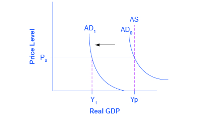
The original Keynesian view using the AD-AS model was that AS was “L”-shaped. At any level of GDP below potential, changes in aggregate demand were thought to have no effect on the price level, only on GDP. Only when GDP reached potential would changes in aggregate demand affect prices, but not GDP. You can see this in the original Keynesian AD-AS model, Figure 1, which we first presented in the module on Keynesian Economics.
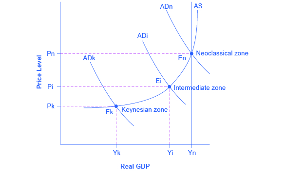
Most Keynesian economists today have a more nuanced view of the AS curve. When the economy is far from potential GDP, changes in AD mostly affect output but not the price level. When the economy is closer to potential GDP, changes in AD affect output and the price level. And when the economy is at or beyond potential GDP changes in AD only affect the price level. This yields the more curved AS that we are familiar with, shown in Figure 2.
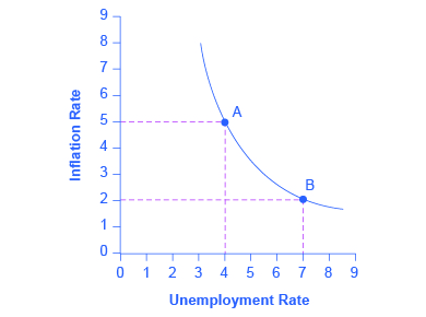
So where does that leave us with the Phillips Curve? Keynesian theory implied that during a recession, when GDP was below potential and unemployment was high, inflationary pressures would be low. Alternatively, when the level of output is at or even pushing beyond potential GDP, the economy is at greater risk for inflation. This yields the Phillips Curve relationship.
Figure 3 shows a theoretical Phillips curve, and the following feature shows how the pattern appears for the United States.
Try It
https://assessments.lumenlearning.co...sessments/7659
https://assessments.lumenlearning.co...sessments/7660
The PHILLIPS CURVE FOR THE UNITED STATES
Step 1. Go to this website to see the 2005 Economic Report of the President.
Step 2. Scroll down and locate Table B-63 in the Appendices. This table is titled “Changes in special consumer price indexes, 1960–2004.”
Step 3. Download the table in Excel by selecting the XLS option and then selecting the location in which to save the file.
Step 4. Open the downloaded Excel file.
Step 5. View the third column (labeled “Year to year”). This is the inflation rate, measured by the percentage change in the Consumer Price Index.
Step 6. Return to the website and scroll to locate the Appendix Table B-42 “Civilian unemployment rate, 1959–2004.
Step 7. Download the table in Excel.
Step 8. Open the downloaded Excel file and view the second column. This is the overall unemployment rate.
Step 9. Using the data available from these two tables, plot the Phillips curve for 1960–69, with unemployment rate on the x-axis and the inflation rate on the y-axis. Your graph should look like Figure 4.
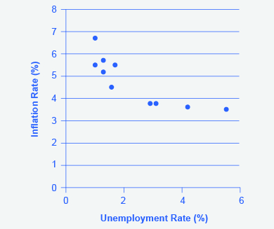
Step 10. Plot the Phillips curve for 1960–1979. What does the graph look like? Do you still see the tradeoff between inflation and unemployment? Your graph should look like Figure 5.
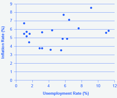
Over this longer period of time, the Phillips curve appears to have shifted out. There is no longer a tradeoff.
The Instability of the Phillips Curve
By the mid-1960s, the Phillips Curve was a key part of Keynesian Economics. The relationship was seen as a policy menu. A nation could choose low inflation and high unemployment, or high inflation and low unemployment, or anywhere in between. Expansionary fiscal and monetary policy could be used to move up the Phillips curve. Contractionary fiscal and monetary policy could be used to move down the Phillips curve. An administration could choose any point on the Phillips Curve as desired.
Then a curious thing happened. When policymakers tried to exploit the tradeoff between inflation and unemployment, the result was an increase in both inflation and unemployment. What had happened? The Phillips curve shifted, but why? The U.S. economy experienced this pattern in the deep recession from 1973 to 1975, and again in back-to-back recessions from 1980 to 1982. Many nations around the world saw similar increases in unemployment and inflation, and this pattern became known as stagflation. (Recall that stagflation is an unhealthy combination of high unemployment and high inflation.) Perhaps most important, stagflation was a phenomenon that could not be explained by traditional Keynesian economics.
Try It
https://assessments.lumenlearning.co...sessments/7657
https://assessments.lumenlearning.co...sessments/7658
watch it
Watch this short video for a summary of the Phillips curve and to learn more about the relationship between inflation and unemployment.
Try It
These questions allow you to get as much practice as you need, as you can click the link at the top of the first question (“Try another version of these questions”) to get a new set of questions. Practice until you feel comfortable doing the questions.
[ohm_question]154506-154508-154519-154523[/ohm_question]
Learning Objectives
[glossary-page]
[glossary-term]contractionary fiscal policy: [/glossary-term]
[glossary-definition]tax increases or cuts in government spending designed to decrease aggregate demand and reduce inflationary pressures [/glossary-definition][glossary-term]expansionary fiscal policy: [/glossary-term][glossary-definition]tax cuts or increases in government spending designed to stimulate aggregate demand and move the economy out of recession[/glossary-definition][glossary-term]Phillips curve:[/glossary-term][glossary-definition]the tradeoff between unemployment and inflation[/glossary-definition][glossary-term]Stagflation: [/glossary-term][glossary-definition]a simultaneous increase in between unemployment and inflation[/glossary-definition]
[/glossary-page]
Contributors and Attributions
- Modification, adaptation, and original content. Provided by: Lumen Learning. License: CC BY: Attribution
- The Phillips Curve. Authored by: OpenStax College. Provided by: Rice University. Located at: https://cnx.org/contents/vEmOH-_p@4.39:H_swtuep@5/The-Phillips-Curve. License: CC BY: Attribution. License Terms: Download for free at http://cnx.org/contents/bc498e1f-efe...569ad09a82@4.4
- The Phillips Curve - 60 Second Adventures in Economics. Provided by: OpenLearn from The Open University. Located at: https://www.youtube.com/watch?v=H_LHFs_Htak&index=3&list=PLhQpDGfX5e7DDGEQvLonjDQsbclAF2N-t. License: Other. License Terms: Standard YouTube License