
8.8: Pivot Tables
- Page ID
- 46545
\( \newcommand{\vecs}[1]{\overset { \scriptstyle \rightharpoonup} {\mathbf{#1}} } \)
\( \newcommand{\vecd}[1]{\overset{-\!-\!\rightharpoonup}{\vphantom{a}\smash {#1}}} \)
\( \newcommand{\id}{\mathrm{id}}\) \( \newcommand{\Span}{\mathrm{span}}\)
( \newcommand{\kernel}{\mathrm{null}\,}\) \( \newcommand{\range}{\mathrm{range}\,}\)
\( \newcommand{\RealPart}{\mathrm{Re}}\) \( \newcommand{\ImaginaryPart}{\mathrm{Im}}\)
\( \newcommand{\Argument}{\mathrm{Arg}}\) \( \newcommand{\norm}[1]{\| #1 \|}\)
\( \newcommand{\inner}[2]{\langle #1, #2 \rangle}\)
\( \newcommand{\Span}{\mathrm{span}}\)
\( \newcommand{\id}{\mathrm{id}}\)
\( \newcommand{\Span}{\mathrm{span}}\)
\( \newcommand{\kernel}{\mathrm{null}\,}\)
\( \newcommand{\range}{\mathrm{range}\,}\)
\( \newcommand{\RealPart}{\mathrm{Re}}\)
\( \newcommand{\ImaginaryPart}{\mathrm{Im}}\)
\( \newcommand{\Argument}{\mathrm{Arg}}\)
\( \newcommand{\norm}[1]{\| #1 \|}\)
\( \newcommand{\inner}[2]{\langle #1, #2 \rangle}\)
\( \newcommand{\Span}{\mathrm{span}}\) \( \newcommand{\AA}{\unicode[.8,0]{x212B}}\)
\( \newcommand{\vectorA}[1]{\vec{#1}} % arrow\)
\( \newcommand{\vectorAt}[1]{\vec{\text{#1}}} % arrow\)
\( \newcommand{\vectorB}[1]{\overset { \scriptstyle \rightharpoonup} {\mathbf{#1}} } \)
\( \newcommand{\vectorC}[1]{\textbf{#1}} \)
\( \newcommand{\vectorD}[1]{\overrightarrow{#1}} \)
\( \newcommand{\vectorDt}[1]{\overrightarrow{\text{#1}}} \)
\( \newcommand{\vectE}[1]{\overset{-\!-\!\rightharpoonup}{\vphantom{a}\smash{\mathbf {#1}}}} \)
\( \newcommand{\vecs}[1]{\overset { \scriptstyle \rightharpoonup} {\mathbf{#1}} } \)
\( \newcommand{\vecd}[1]{\overset{-\!-\!\rightharpoonup}{\vphantom{a}\smash {#1}}} \)
\(\newcommand{\avec}{\mathbf a}\) \(\newcommand{\bvec}{\mathbf b}\) \(\newcommand{\cvec}{\mathbf c}\) \(\newcommand{\dvec}{\mathbf d}\) \(\newcommand{\dtil}{\widetilde{\mathbf d}}\) \(\newcommand{\evec}{\mathbf e}\) \(\newcommand{\fvec}{\mathbf f}\) \(\newcommand{\nvec}{\mathbf n}\) \(\newcommand{\pvec}{\mathbf p}\) \(\newcommand{\qvec}{\mathbf q}\) \(\newcommand{\svec}{\mathbf s}\) \(\newcommand{\tvec}{\mathbf t}\) \(\newcommand{\uvec}{\mathbf u}\) \(\newcommand{\vvec}{\mathbf v}\) \(\newcommand{\wvec}{\mathbf w}\) \(\newcommand{\xvec}{\mathbf x}\) \(\newcommand{\yvec}{\mathbf y}\) \(\newcommand{\zvec}{\mathbf z}\) \(\newcommand{\rvec}{\mathbf r}\) \(\newcommand{\mvec}{\mathbf m}\) \(\newcommand{\zerovec}{\mathbf 0}\) \(\newcommand{\onevec}{\mathbf 1}\) \(\newcommand{\real}{\mathbb R}\) \(\newcommand{\twovec}[2]{\left[\begin{array}{r}#1 \\ #2 \end{array}\right]}\) \(\newcommand{\ctwovec}[2]{\left[\begin{array}{c}#1 \\ #2 \end{array}\right]}\) \(\newcommand{\threevec}[3]{\left[\begin{array}{r}#1 \\ #2 \\ #3 \end{array}\right]}\) \(\newcommand{\cthreevec}[3]{\left[\begin{array}{c}#1 \\ #2 \\ #3 \end{array}\right]}\) \(\newcommand{\fourvec}[4]{\left[\begin{array}{r}#1 \\ #2 \\ #3 \\ #4 \end{array}\right]}\) \(\newcommand{\cfourvec}[4]{\left[\begin{array}{c}#1 \\ #2 \\ #3 \\ #4 \end{array}\right]}\) \(\newcommand{\fivevec}[5]{\left[\begin{array}{r}#1 \\ #2 \\ #3 \\ #4 \\ #5 \\ \end{array}\right]}\) \(\newcommand{\cfivevec}[5]{\left[\begin{array}{c}#1 \\ #2 \\ #3 \\ #4 \\ #5 \\ \end{array}\right]}\) \(\newcommand{\mattwo}[4]{\left[\begin{array}{rr}#1 \amp #2 \\ #3 \amp #4 \\ \end{array}\right]}\) \(\newcommand{\laspan}[1]{\text{Span}\{#1\}}\) \(\newcommand{\bcal}{\cal B}\) \(\newcommand{\ccal}{\cal C}\) \(\newcommand{\scal}{\cal S}\) \(\newcommand{\wcal}{\cal W}\) \(\newcommand{\ecal}{\cal E}\) \(\newcommand{\coords}[2]{\left\{#1\right\}_{#2}}\) \(\newcommand{\gray}[1]{\color{gray}{#1}}\) \(\newcommand{\lgray}[1]{\color{lightgray}{#1}}\) \(\newcommand{\rank}{\operatorname{rank}}\) \(\newcommand{\row}{\text{Row}}\) \(\newcommand{\col}{\text{Col}}\) \(\renewcommand{\row}{\text{Row}}\) \(\newcommand{\nul}{\text{Nul}}\) \(\newcommand{\var}{\text{Var}}\) \(\newcommand{\corr}{\text{corr}}\) \(\newcommand{\len}[1]{\left|#1\right|}\) \(\newcommand{\bbar}{\overline{\bvec}}\) \(\newcommand{\bhat}{\widehat{\bvec}}\) \(\newcommand{\bperp}{\bvec^\perp}\) \(\newcommand{\xhat}{\widehat{\xvec}}\) \(\newcommand{\vhat}{\widehat{\vvec}}\) \(\newcommand{\uhat}{\widehat{\uvec}}\) \(\newcommand{\what}{\widehat{\wvec}}\) \(\newcommand{\Sighat}{\widehat{\Sigma}}\) \(\newcommand{\lt}{<}\) \(\newcommand{\gt}{>}\) \(\newcommand{\amp}{&}\) \(\definecolor{fillinmathshade}{gray}{0.9}\)Learning Objectives
- Pivot tables
In Excel, the PivotTable tool creates ways to reorganize data in a spreadsheet. Reorganizing data in this way, brings about additional information and insights that foster better understanding of your data. PivotTables allow you to forgo creating many summary calculations by hand, because a PivotTable does the work for you.
The example below includes a multicolumn table of sales data containing just over a year’s worth of information. Looking at the raw data in the table you may be able to pull out a few salient points, but with a pivot table, you can quickly answer questions like:
- What was the largest order by sales or by product quantity?
- What was the grand total sold of furniture for 2019 per region?
- Which sales region had the lowest sales figures?
- What sales representative had the highest total sales?

Practice Question
Now that you understand that PivotTables can be a powerful assistant with your Excel data, let’s look at a few examples and the two main ways to create a PivotTable; the Recommended PivotTable button, or by creating a PivotTable from scratch.
Create by Recommend PivotTables Button
If you are unfamiliar with pivot tables, this process is the recommended option to use until you become more familiar with them. The dialog box displays various options for a given data set, giving you a range of choices so you can select the one best suited for your data analysis.
Follow these steps to use this tool:
- Open an Excel spreadsheet with existing data, click on any cell within the data table and click the Insert tab.
- Click the Recommended PivotTables button in the Tables group. The entire table has been selected, indicated by the dotted line around the border of the data table.
- Alternative short-cut for data selection if the data set is large: While holding down the Shift + Ctrl keys, tap the right arrow key on your keyboard. Then while still holding down the Shift + Ctrl keys, click the down arrow key on the keyboard. All the data should now be selected in the entire data table.
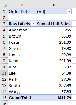
- In the Recommended Pivot Tables window, a variety of Pivot Tables are available to be selected. Scroll through the options, select one and click OK. In this example, the Sum of Unit Sale by Region is selected.

Note
If you decide at this point a blank PivotTable is preferable, select the Blank PivotTable button on the bottom left.
- A new tab is opened containing the information of the selected PivotTable. Notice that the PivotTable will calculate the sum of unit sales per region in the table that was selected even without any of the total cost column filled out in the original data table.

- This new PivotTable, summing up the sales, is the first step in rearranging the original data to be able to take a more in-depth analysis of the data. You can stop here or repeat the process and create other recommended tables.
- If an additional PivotTable is desired, such as sales per sales rep, or sum of unit sales per item and region, return to tab containing the original data, follow the same steps using the Recommended PivotTables button, scroll until you see the desired table, and select it. Here are two other examples of PivotTables created from the same data set.
Create by PivotTables Button
If you are more familiar with pivot tables, or simply wish to create one from the ground up, this button allows you select and reorganize the data however you want to see the data interpreted. Follow these steps to create a PivotTable from scratch.
- Open an Excel worksheet containing data for the PivotTable tool and select a cell anywhere in the data set.
- Click the Insert tab, and the PivotTable button on the ribbon. Excel will automatically select the data it identifies as the information for this table.
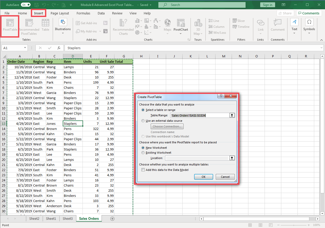
- If the selected area missed data, start again by clicking on the beginning data table cell, drag the cursor over all the desired data to select. Once the area is selected, click the PivotTable button under the Insert tab, Tables Group.
- Another option to select the correct table data: Click on the PivotTable button and open the Create PivotTable dialog box. In the box under the “Choose the data you want to analyze” area, type in the table/range area for the table; for example ‘Sales Orders’!$A$1:$G$4, or drag the cursor over the data area for the table and the range will be added to the Table/Range field.
- After making sure the data selected is correct, select New Worksheet option, and click the OK.
- A new worksheet is created. On the right side of the worksheet, a PivotTable Fields task pane is open. In it are four areas (Filters, Columns, Rows, and Values) where various field names can be placed to create a PivotTable. The task pane also includes a checklist area of the fields from which to choose from the data.
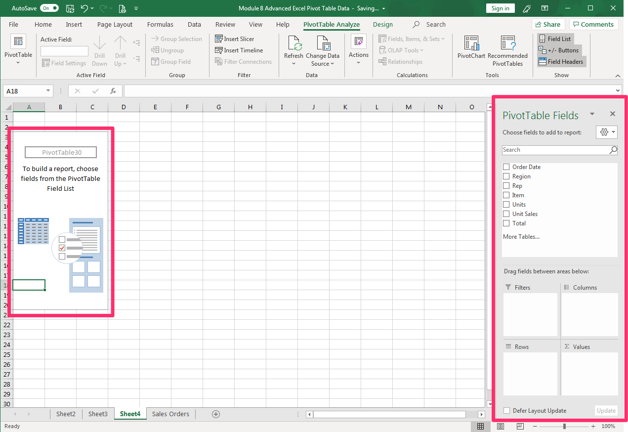
- Drag one field name into different areas to create a PivotTable. Alternatively, you can check the boxes for fields to be added to the table. Each of the areas operate in the following manner in a PivotTable:
- Columns: The filed used to measure and compare data.
- Rows: The field for data you want to analyze.
- Values: The field containing the values a table uses for comparisons.
- Filter (optional): A field used to sort table data. It is displayed in the upper left corner of a table and is an optional field for tables.
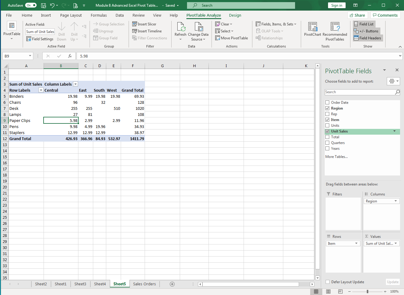
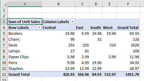
- The PivotTable in the screenshot above is created based on the sales data of these fields added to these areas:
- Columns: Region
- Rows: Item
- Values: Sum of Unit Sales
- Rearrange fields in a variety of ways by dragging them into a new area or clicking the option in the list of fields above the areas. Each action will affect the PivotTable. Move fields around into new areas until you have created a table giving you the best insight into your data. Congratulations! You have created a PivotTable from scratch.
Note
You may run into scenarios where a data field is dragged into an area that does not work well. Simply drag the field into another area and quickly see whether that field in the new area works better. Excel made the PivotTable tool flexible so you can easily change the structure of fields and areas if you make a misstep along the way.
Practice Question
Contributors and Attributions
- Pivot Tables. Authored by: Sherri Pendleton. Provided by: Lumen Learning. License: CC BY: Attribution