6.1: High-Low Method

Last updated
Save as PDF

Page ID: 45858

$ \newcommand{\vecs}[1]{\overset { \scriptstyle \rightharpoonup} {\mathbf{#1}} } $ $ \newcommand{\vecd}[1]{\overset{-\!-\!\rightharpoonup}{\vphantom{a}\smash {#1}}} $$\newcommand{\id}{\mathrm{id}}$ $ \newcommand{\Span}{\mathrm{span}}$ $ \newcommand{\kernel}{\mathrm{null}\,}$ $ \newcommand{\range}{\mathrm{range}\,}$ $ \newcommand{\RealPart}{\mathrm{Re}}$ $ \newcommand{\ImaginaryPart}{\mathrm{Im}}$ $ \newcommand{\Argument}{\mathrm{Arg}}$ $ \newcommand{\norm}[1]{\| #1 \|}$ $ \newcommand{\inner}[2]{\langle #1, #2 \rangle}$ $ \newcommand{\Span}{\mathrm{span}}$ $\newcommand{\id}{\mathrm{id}}$ $ \newcommand{\Span}{\mathrm{span}}$ $ \newcommand{\kernel}{\mathrm{null}\,}$ $ \newcommand{\range}{\mathrm{range}\,}$ $ \newcommand{\RealPart}{\mathrm{Re}}$ $ \newcommand{\ImaginaryPart}{\mathrm{Im}}$ $ \newcommand{\Argument}{\mathrm{Arg}}$ $ \newcommand{\norm}[1]{\| #1 \|}$ $ \newcommand{\inner}[2]{\langle #1, #2 \rangle}$ $ \newcommand{\Span}{\mathrm{span}}$$\newcommand{\AA}{\unicode[.8,0]{x212B}}$

Learning Outcomes

Analyze mixed costs using the high-low method

In our previous dog groomer example we could clearly see through our scattergram that maintenance costs were related to the number of dogs groomed. Remember that that was our initial diagnostic step before we moved on to more detailed analysis of our costs.

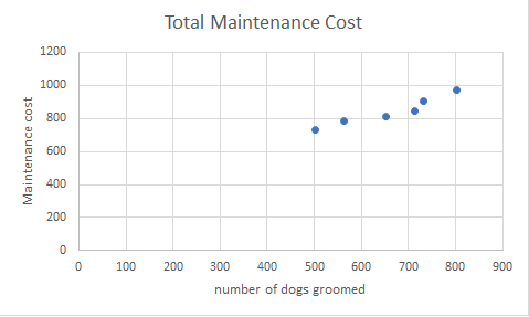
A graph showing total maintenance cost with number of dogs groomed on the x-axis and maintenance cost on the y-axis. As the number of dogs groomed increases, maintenance cost increases.

The scattergram above shows a relatively linear relationship between the maintenance costs (cost-Y) and the number of dogs groomed (activity -X) we can use the high-low method to estimate which portion of our expense is the fixed portion and which is the variable portion.

With this method we first look for the period with the lowest level of activity and the highest level. Going back to our chart from 7.2.2 the lowest month 500 dogs were groomed and the maintenance cost was $740. The highest month 800 dogs were groomed and the maintenance cost was $980. Now we can use those numbers in our high-low formula:

Variable cost = Cost at the high activity level-cost at the low level of activity

High activity level − Low activity level

Variable cost = Change in cost

Change in activity

Variable cost = $980 − $740

800 − 500

Variable cost = $240/300 or .80 for each dog groomed

We can now calculate the fixed cost component. We can use the total cost of either the high or the low and subtract the variable component:

Fixed cost = Total cost − Variable cost element

Fixed cost= $980 − .8(800) = $980 − $640 = $340 using the highest month

Fixed cost = $740 − .8(500) = $740 − $400= $340 using the lowest month

Note

This method can only be used if the scattergram that you used for your initial testing shows a linear correlation between the costs and the quantity! Also note that although this method is simple to apply it only uses the two points of data. Having only two points of data might produce results that are not accurate. Because of this, the next section on the least squares regression will probably be more useful and reliable for determining the fixed and variable portions of mixed costs.

Practice Questions

https://assessments.lumenlearning.co...sessments/9602

High-Low Method. Authored by: Freedom Learning Group. Provided by: Lumen Learning. License: CC BY: Attribution