20: Yield Curves

Last updated
Save as PDF

Page ID: 12765

$ \newcommand{\vecs}[1]{\overset { \scriptstyle \rightharpoonup} {\mathbf{#1}} } $ $ \newcommand{\vecd}[1]{\overset{-\!-\!\rightharpoonup}{\vphantom{a}\smash {#1}}} $$\newcommand{\id}{\mathrm{id}}$ $ \newcommand{\Span}{\mathrm{span}}$ $ \newcommand{\kernel}{\mathrm{null}\,}$ $ \newcommand{\range}{\mathrm{range}\,}$ $ \newcommand{\RealPart}{\mathrm{Re}}$ $ \newcommand{\ImaginaryPart}{\mathrm{Im}}$ $ \newcommand{\Argument}{\mathrm{Arg}}$ $ \newcommand{\norm}[1]{\| #1 \|}$ $ \newcommand{\inner}[2]{\langle #1, #2 \rangle}$ $ \newcommand{\Span}{\mathrm{span}}$ $\newcommand{\id}{\mathrm{id}}$ $ \newcommand{\Span}{\mathrm{span}}$ $ \newcommand{\kernel}{\mathrm{null}\,}$ $ \newcommand{\range}{\mathrm{range}\,}$ $ \newcommand{\RealPart}{\mathrm{Re}}$ $ \newcommand{\ImaginaryPart}{\mathrm{Im}}$ $ \newcommand{\Argument}{\mathrm{Arg}}$ $ \newcommand{\norm}[1]{\| #1 \|}$ $ \newcommand{\inner}[2]{\langle #1, #2 \rangle}$ $ \newcommand{\Span}{\mathrm{span}}$$\newcommand{\AA}{\unicode[.8,0]{x212B}}$

Learning Objectives

After completing this chapter, you should be able to: (1) understand how interest and earning rates on a variety of debt and investments instruments are related to yield curves and periodic interest rates; (2) describe how yield curves and periodic interest rates defined over future time periods can be used to predict market participants’ expectation of future opportunities and threats; and (3) use yield curves and periodic interest rates to better understand and predict future financial opportunities and threats.

To achieve your learning goals, you should complete the following objectives.

Learn how to calculate single period discount rates from investments of varying terms.
Understand the relationship between yield curves and single period discount rates.
Learn how yield curves can be used to predict future financial opportunities and threats.

Introduction

In most present value (PV) models, the discount rate is a constant even when the term of the model has changed. In reality, each period’s discount rate may be different because factors that influence the discount rate are not constant. These factors include the level of economic growth in the economy, the inflation rate, national and international events likely to influence our economy, activities in the stock and bond market, housing and land markets, the unemployment rate, and election outcomes.

One way to observe the difference in period discount rates is to observe the interest rates on loans with different terms. They are not constant. To demonstrate, note the changes in variable interest rate loans. They aren’t constant either. Or, relevant to this discussion, notice the difference in average yields on bonds with different maturities even in the same risk class. Alternatively, notice the change in the internal rate of return (IRR) of a bond as its time to maturity changes over times.

In what follows, we pursue two objectives. The first objective is to demonstrate how to calculate the periodic discount rate for no-coupon bonds. The approach we describe can also be used to find periodic discount rates implied by bonds that are more complicated as well as other financial instruments. Our second objective is to connect the shapes and patterns of periodic interest rate curves and their corresponding yield curves patterns to predict future economic activity and opportunities and threats. Yield curves, as we will explain in more detail later, are the geometric means of periodic interest rates at a point in time with various maturities.

Geometric Means and Periodic Discount Rates

Geometric means and long-term discount rates. Suppose we have information that allows us to predict n future periodic discount rates r₁, r₂, ⋯, r_n. The geometric mean for the n periodic rates satisfies the following equation:

(20.1) quicklatex.com-af16c7a543f3932b37b2b8afa0355100_l3.png

In words, one plus the geometric mean multiplied by itself n times would equal the product of 1 plus n periodic discount rates. We can solve for the geometric mean of the n periodic discount rates in Equation \ref{20.1} by finding the nth root of the products of the n periodic discount rates and subtracting one:

(20.2) $n)} -1 \end{equation*}$

To demonstrate, suppose that periodic discount rates for period one through three were r₁ = .07, r₂ = .03, and r₃ = .075. We can solve for the geometric mean of the three periodic interest rates as:

(20.3) $3)} -1 = .058\, or\, 5.8\% \end{equation*}$

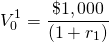
How to calculate periodic discount rates. Consider a zero coupon bond that can be purchased for quicklatex.com-f99551c5f893d4d6389e591cbe500cc4_l3.png at the beginning of the period and redeemed at the end of the period for its par value of $1,000. The periodic rate of return r₁ for the one-period bond satisfies the PV model:

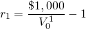
(20.4) quicklatex.com-c8bc083b8e43b74797683dcc0473e889_l3.png

Solving for the one-period discount rate r₁ we find:

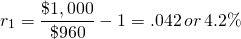
(20.5) quicklatex.com-e720e92af7d61e09f108335fe4dc8b21_l3.png

For example if quicklatex.com-42fe5f221b9a064321f03070f1ab43d0_l3.png then

(20.6) quicklatex.com-ae4ae4129bd9a2dbd5687b8bd1960823_l3.png

In the case of a one-period bond, the one-period discount rate is also the geometric mean.

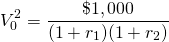
Now consider a zero-coupon bond that matures in two periods with similar risk and tax provisions as the one-period bond described in Equation \ref{20.4}. Assume the zero-coupon two-period bond can be purchased for quicklatex.com-8778b725d71c73cfea0f70ed259b9753_l3.png at the beginning of the period and redeemed at the end of the period for its par value of $1,000. The periodic rate of return r₂ for the two-period bond satisfies the PV model:

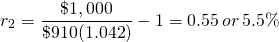
(20.7) quicklatex.com-50ff677db6ca995dfcdc29e23f24ae16_l3.png

Solving for the second period discount rate r₂ we find:

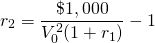
(20.8) quicklatex.com-2b8685ffbdf6009ea902bec3a59fb41a_l3.png

For example if quicklatex.com-c13d0eaa5f97a9da53557eae3770eb6b_l3.png then

(20.9) quicklatex.com-bcdef1c092524cfbd19ef0623772a5e6_l3.png

When we purchase a two period bond, we acquire a financial instrument with a single yield for two periods. The yield is the geometric mean of the product of the single period discount rates. In our example, the yield or geometric mean is equal to:

(20.10) $2} -1 = .048 \,or\, 4.8\% \end{equation*}$

Continuing our example, if quicklatex.com-220a5b4d009fe661f17f332559b5dbce_l3.png then

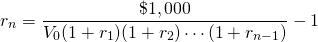
(20.11) quicklatex.com-bb71fd583e495bd5335614b20e98cf3f_l3.png

Finally, consider a zero-coupon n period bond that can be purchased for quicklatex.com-a4fc13a061f828cc3d2078665519a36f_l3.png at the beginning of the period and redeemed at the end of the period for its par value of $1,000. The periodic rate of return r_n for the n period bond satisfies the PV model equal to:

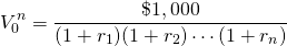
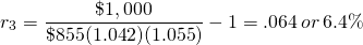
(20.12) quicklatex.com-ca73311a40dae8ded0d0edde91e16907_l3.png

Solving for the one-period discount rate r_n we find:

(20.13) quicklatex.com-e3a5c66ec8ac6f87a8fd02275b1d676e_l3.png

Periodic rates of return and geometric means. When we purchase a three-period bond, we acquire a single yield for three periods. Consistent with the PV model, the yield is the geometric mean of the product of the single-period discount rates. In our example, the yield or geometric mean for the three-period bond is equal to:

(20.14) $3} -1 = .054 \, or \, 5.4\% \end{equation*}$

While one could expect to earn the bond’s yield to maturity if the investor held the bond to maturity, a three-year bond becomes a two-year bond after one year, and if sold, the bond’s price would reflect the yield on a two-year bond.

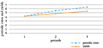
Graphing the geometric means of bonds against their varying time to maturity produces the bond’s yield curve. In Figure 20.1, we graph the periodic discount rates and the corresponding yield curves for one, two, and three period bonds.

Figure 20.1. A comparison of periodic interest rates and the corresponding yield curves of bonds of varying maturities

Predicting Future Economic Activities and Opportunities and Threats

Marginal periodic rates and average geometric mean yield curves. The periodic rate is a marginal rate while the yield rate is an average or mean—in this case a geometric mean. In our example, the periodic rate is increasing. As a result, the yield curve is also increasing but at a slower rate because previous and lower values of the periodic rate influence the yield. Therefore, if the yield curve is increasing, it is because the marginal periodic rates added to the series are greater than the geometric mean of the previous values included in the calculation. Moreover, if the yield curve were decreasing, it would require that periodic rates added were less than the geometric mean. To be complete, if the yield curve were constant, it would suggest that the marginal periodic rate were equal to the geometric mean.

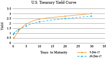
Of course, there are many bond yield curves depending on the type of bond considered. When producing a yield curve, it is essential that bonds used to produce the yield curve belong to a similar risk class—even though this may be difficult because term differences produce different risks. To do the best we can to hold risk constant when producing yield curves, government backed debt is often considered. The most frequently reported yield curve compares three-month, two-year, five-year and thirty-year U.S. Treasury debt. We present graphs of U.S. Treasury yield curves at two points in time in Figure 20.2 below

Figure 20.2. Yield curves using U.S. Treasury debt calculated on January 3, 2017 and June 20, 2017

Interpreting the shapes of yield curves. In the previous section, we described the relationship between the period or marginal interest rates and the yield curve that, according to our PV model, is the geometric mean of the periodic rates. We now suggest some interpretations of the yield curves. Figures of periodic rate calculated from yield curves are not generally available.

Positively sloped yield curves. To invest or lend one’s financial capital to another person or entity requires a sacrifice on the part of the lender. Furthermore, the longer the funds are committed to another person or entity, the greater is the sacrifice. As a result, many economists claim that upward sloping yield curves predict a healthy economy in the future where borrowers have a bright view of future earnings and are willing to pay increased interest rates for the privilege of investing in the future. Another explanation is that borrowers expect periodic interest rates in the future to rise that in turn will produce an increasing yield curve. One reason for periodic rates to rise is expected increases in inflation and subsequent response to inflation by the Federal Reserve to increase interest rates on government debt instruments to offset inflationary pressures.
Flat or humped yield curves. A flat yield curve is consistent with constant periodic interest rates so that all bond maturities have similar yields. A humped yield curve implies that periodic interest rates for a period lie above then fall below the yield curve and are constant before and after the hump. Economists generally view constant or humped yield curves as uncertain indicators of the future well-being of the economy.
Negatively sloped or inverted yield curves. During periods when financial market participants expect periodic rates of return to decrease, yield curves have been downward sloping or inverted. Some financial economist connect inverted yield curves with pending downturns in the economy or recessions. In support of this connection, an inverted yield curve has indicated a worsening economic situation in the future 7 times since 1970 (Adrian, 2010). See Table 20.1.

Summary and Conclusions

Previous chapters have treated the multi-period discount rate in PV models (including IRR) as constants. This chapter has emphasized that these constant discount rates are composed of time varying periodic discount rates. Many time-varying factors would prevent periodic discount rates from being constant. Such forces acting on periodic interest rates include monetary and fiscal policies, inflation rates, unemployment rates, and national and international trade and treaties to name a few.

So what have we learned? We learned that rate of return expectations built into periodic discount rates and reflected in yield curves of bonds (and interest rates) of varying maturities reflect expected future economic conditions.

While there is not universal agreement on how to interpret yield curves, and indeed different yield curves may be subject to varying interpretations, there is support for interpreting downward sloping or inverted yield curves as foreshadowing a slow-down in future economic activities.

The goal of this chapter has been to acquaint students with another resource for predicting future opportunities and threats.

Table 20.1. The connection between inverted yield curves and future recessions (1970-2009).

Event	Date of Inversion Start	Date of the Recession Start	Time from Inversion to Recession Start	Duration of Inversion	Duration of Recession
Event	Date of Inversion Start	Date of the Recession Start	Months	Months	Months
1970 Recession	Dec-68	Jan-70	13	15	11
1974 Recession	Jun-73	Dec-73	6	18	16
1980 Recession	Nov-78	Feb-80	15	18	6
1981–1982 Recession	Oct-80	Aug-81	10	12	16
1990 Recession	Jun-89	Aug-90	14	7	8
2001 Recession	Jul-00	1-Apr	9	7	8

Questions

Compare geometric means and periodic discount rates.
Find the geometric mean of three periodic discount rates equal to .
Suppose the geometric mean of two periodic discount rates was 6%, and the periodic discount rate in the second period was 7%. Find the periodic discount rate in the first period.
Suppose a one-year zero-coupon bond with a par value of $1,000 was selling for $962. Find the bond’s yield.
Suppose the yield curve was decreasing. Some economics would view this as a sign the economy is slowing down. Do you agree or disagree? Defend your answer.
Find data on the yield curve in the economy and discuss what it portends.