10.9: Fixed Manufacturing Overhead Variance Analysis
- Page ID
- 2073
- Calculate and analyze fixed manufacturing overhead variances.
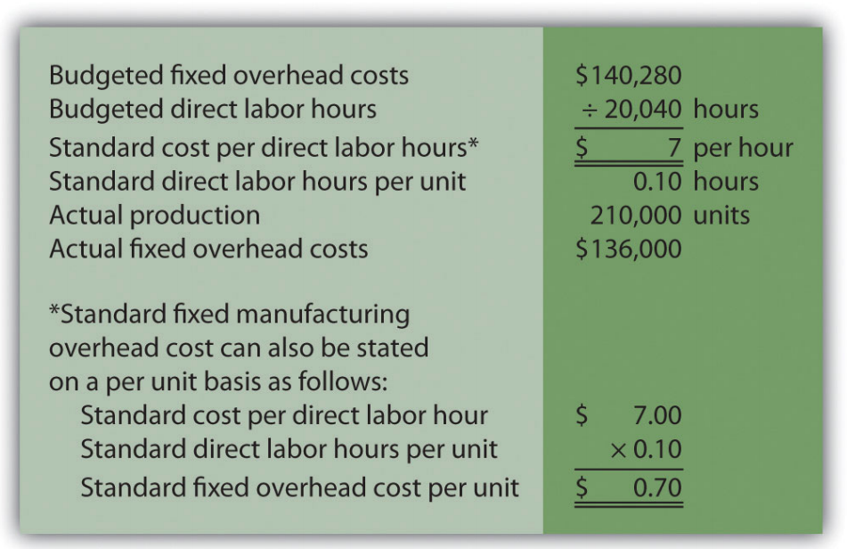
Question: Many organizations also analyze fixed manufacturing overhead variances. Recall from earlier chapters that manufacturing companies are required to assign fixed manufacturing overhead costs to products for financial reporting purposes (this is called absorption costing). It is common for companies such as Jerry’s Ice Cream to apply fixed manufacturing overhead costs to products based on direct labor hours, machine hours, or some other activity. Companies using a standard costing system apply fixed overhead based on a standard dollar amount per unit produced (this calculation is shown in the footnote to Figure 10.12). Assume Jerry’s uses direct labor hours to assign fixed overhead costs to products shown in Figure 10.12. How is this information used to perform fixed overhead cost variance analysis?
- Answer
-
It is important to start by noting that fixed overhead in the master budget is the same as fixed overhead in the flexible budget because, by definition, fixed costs do not change with changes in units produced. Thus budgeted fixed overhead costs of $140,280 shown in Figure 10.12 will remain the same even though Jerry’s actually produced 210,000 units instead of the master budget expectation of 200,400 units.

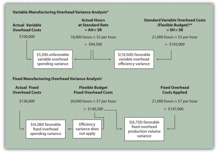
Figure \(\PageIndex{12}\): - Fixed Manufacturing Overhead Information for Jerry’s Ice Cream Fixed manufacturing overhead variance analysis involves two separate variances: the spending variance and the production volume variance. We show both variances in Figure 10.13, and provide further detail following the figure.

Figure \(\PageIndex{13}\): - Fixed Manufacturing Overhead Variance Analysis for Jerry’s Ice Cream *From Chapter 9, the direct labor budget is 20,040 budgeted direct labor hours = 200,400 units budgeted to be produced × 0.10 direct labor hours per unit.
**Standard hours of 21,000 = 210,000 actual units produced and sold × Standard of 0.10 hours per unit.
† $140,280 is the original budget presented in the manufacturing overhead budget shown in Chapter 9. The flexible budget amount for fixed overhead does not change with changes in production, so this amount remains the same regardless of actual production.
‡ $(4,280) favorable fixed overhead spending variance = $136,000 – $140,280. Variance is favorable because the actual fixed overhead costs are lower than the budgeted costs.
§ $(6,720) favorable fixed overhead volume variance = $140,280 – $147,000. Variance is favorable because the volume of goods produced and sold was higher than expected.
Fixed Overhead Spending Variance Calculation
Question: How is the fixed overhead spending variance calculated?
- Answer
-
The fixed overhead spending variance21 is the difference between actual and budgeted fixed overhead costs. As shown in Figure 10.13, Jerry’s Ice Cream incurred $136,000 in fixed overhead costs for the year. Budgeted fixed overhead costs totaled $140,280. Thus the spending variance is calculated as follows:
\[\text{Fixed overhead spending variance}\; = \text{Actual costs} - \text{Budgeted costs}\]
\[\begin{split} \text{Fixed overhead spending variance} &= \text{Actual costs} - \text{Budgeted costs} \\ &= \$136,000 - $140,280 \\ &= (\$ 4,280)\quad \text{favorable} \end{split}\]
Because fixed overhead costs are not typically driven by activity, Jerry’s cannot attribute any part of this variance to the efficient (or inefficient) use of labor. In fact, there is no efficiency variance for fixed overhead. Instead, Jerry’s must review the detail of actual and budgeted costs to determine why the favorable variance occurred. For example, factory rent, supervisor salaries, or factory insurance may have been lower than anticipated. Further investigation of detailed costs is necessary to determine the exact cause of the fixed overhead spending variance.
Fixed Overhead Production Volume Variance Calculation
Question: How is the fixed overhead production volume variance calculated?
- Answer
-
Before discussing the production volume variance, a word of caution: do not equate the fixed overhead production volume variance with the variable overhead efficiency variance. There is no efficiency variance for fixed manufacturing overhead because, by definition, fixed costs do not change with changes in the activity base. The fixed overhead volume variance is solely a result of the difference in budgeted production and actual production. The fixed overhead production volume variance22 is the difference between the budgeted and applied fixed overhead costs. As shown in Figure 10.13, Jerry’s Ice Cream budgeted $140,280 in fixed overhead costs for the year. Fixed overhead costs applied totaled $147,000. Thus the production volume variance is calculated as follows:
\[\text{Fixed overhead production volume variance}\; = \text{Budgeted costs} - \text{Applied costs}\]
\[\begin{split} \text{Fixed overhead production volume variance}\; &= \text{Budgeted costs} - \text{Applied costs} \\ &= \$ 140,280 - \$ 147,000 \\ &= (\$ 6,720)\quad \text{favorable} \end{split}\]
The fixed overhead production volume variance is a direct result of the difference in volume (units) between budgeted production and actual production. All other variables are held constant including standard direct labor hours per unit (0.10) and standard rate per direct labor hour ($7). Thus an alternative approach to this calculation can be used assuming the standard fixed overhead cost per unit is $0.70 (= 0.10 direct labor hours per unit × $7 per direct labor hour):
\[\text{Fixed overhead production volume variance}\; = \text{Standard fixed overhead cost per unit} \times \text{Budgeted units produced}\]
\[\begin{split} \text{Fixed overhead production volume variance}\; &= \text{Standard fixed overhead cost per unit} \times \text{Budgeted units produced} \\ (\$ 6,720)\quad \text{favorable} &= \$ 0.70 \times 200,400\; \text{budgeted units} \end{split}\]
The fixed overhead production volume variance is favorable because the company produced and sold more units than anticipated.
Comparison of Fixed and Variable Overhead Variances
Question: What are the similarities and differences between the fixed and variable overhead variances?
- Answer
-
Figure 10.14 summarizes the similarities and differences between variable and fixed overhead variances. Notice that the efficiency variance is not applicable to the fixed overhead variance analysis.

Figure \(\PageIndex{14}\): - Comparison of Variable and Fixed Manufacturing Overhead Variance Analysis for Jerry’s Ice Cream *Information is from Figure 10.8.
**For variable manufacturing overhead, the flexible budget is the same as variable overhead applied to production.
† Information is from Figure 10.13
Two variances are calculated and analyzed when evaluating fixed manufacturing overhead. The fixed overhead spending variance is the difference between actual and budgeted fixed overhead costs. The fixed overhead production volume variance is the difference between budgeted and applied fixed overhead costs. There is no efficiency variance for fixed manufacturing overhead.
This review problem is based on the budget information presented in Chapter 9 review problems and variance analysis information presented in Chapter 10 review problems. The following information is for Carol’s Cookies:

- Answer
-

*Standard hours of 78,000 = 390,000 actual units produced and sold x standard of 0.20 hours per unit.
**$5,340 unfavorable fixed overhead spending variance = $270,000 – $264,660. Variance is unfavorable because the actual fixed overhead costs are higher than the budgeted costs.
† $7,260 unfavorable fixed overhead volume variance = $264,660 – $257,400. Variance is unfavorable because the volume of goods produced and sold was lower than expected.
Definitions
- The difference between actual and budgeted fixed overhead costs.
- The difference between the budgeted and applied fixed overhead costs.


