9.18: Costs in the Short Run

Last updated
Save as PDF

Page ID: 48398

$ \newcommand{\vecs}[1]{\overset { \scriptstyle \rightharpoonup} {\mathbf{#1}} } $ $ \newcommand{\vecd}[1]{\overset{-\!-\!\rightharpoonup}{\vphantom{a}\smash {#1}}} $$\newcommand{\id}{\mathrm{id}}$ $ \newcommand{\Span}{\mathrm{span}}$ $ \newcommand{\kernel}{\mathrm{null}\,}$ $ \newcommand{\range}{\mathrm{range}\,}$ $ \newcommand{\RealPart}{\mathrm{Re}}$ $ \newcommand{\ImaginaryPart}{\mathrm{Im}}$ $ \newcommand{\Argument}{\mathrm{Arg}}$ $ \newcommand{\norm}[1]{\| #1 \|}$ $ \newcommand{\inner}[2]{\langle #1, #2 \rangle}$ $ \newcommand{\Span}{\mathrm{span}}$ $\newcommand{\id}{\mathrm{id}}$ $ \newcommand{\Span}{\mathrm{span}}$ $ \newcommand{\kernel}{\mathrm{null}\,}$ $ \newcommand{\range}{\mathrm{range}\,}$ $ \newcommand{\RealPart}{\mathrm{Re}}$ $ \newcommand{\ImaginaryPart}{\mathrm{Im}}$ $ \newcommand{\Argument}{\mathrm{Arg}}$ $ \newcommand{\norm}[1]{\| #1 \|}$ $ \newcommand{\inner}[2]{\langle #1, #2 \rangle}$ $ \newcommand{\Span}{\mathrm{span}}$$\newcommand{\AA}{\unicode[.8,0]{x212B}}$

Learning Objectives

Describe the relationship between production and costs, including average and marginal costs
Analyze short-run costs in terms of fixed cost and variable cost

We’ve explained that a firm’s total cost of production depends on the quantities of inputs the firm uses to produce its output and the cost of those inputs to the firm. The firm’s production function tells us how much output the firm will produce with given amounts of inputs. A production function can be expressed mathematically as

$Q=f\left[L\text{,}\stackrel{-}{K}\right]$

where Q is the firm’s output, L is the amount of labor employed, and K is the amount of fixed capital.

Suppose we think about the production function backwards:

$L=g\left[Q\text{,}\stackrel{-}K\right]$ ,

where the g just means the function f in reverse. This equation tells us how much labor we need to produce a given level of output, with the fixed capital stock we have. If we knew the cost of labor and capital, we could then compute the total cost of producing any level of output. It is to this that we next turn.

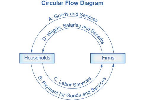
For every factor of production (or input), there is an associated factor payment. Factor payments are what the firm pays for the use of the factors of production. From the firm’s perspective, factor payments are costs. From the owner of each factor’s perspective, factor payments are income. Factor payments include:

The circular flow diagram’s outer arrows represent a goods and services market, and the inner arrows represent a labor market. As illustrated by the outer arrows, in a goods and services market, firms give goods and services to households and, in exchange, households give payment to firms. As illustrated by the inner arrows, in a labor market, households provide labor to firms and, in exchange, firms give wages, salaries, and benefits to households.

Figure 1. The Circular Flow Diagram is a model of economic activity with firms supplying goods and services (arrow A) to households. In return, households pay for those goods and services (arrow B). The inner circle of arrows shows factors and factor payments. In this figure, household supply labor services (arrow C) to firms, who pay wages, salaries and benefits (arrow D) in return. A more complete model would include all the other factors supplied in arrow C, and the associated factor payments in arrow D.

Raw materials prices for raw materials
Rent for land or buildings
Wages and salaries for labor
Interest and dividends for the use of financial capital (loans and equity investments)
Profit for entrepreneurship. Profit is the residual, what’s left over from revenues after the firm pays all the other costs. While it may seem odd to treat profit as a “cost”, it is the payment that goes from total revenues to entrepreneurs or taking the risk of starting a business. You can see this correspondence between factors of production and factor payments in the inside loop of the circular flow diagram in Figure 1.

We now have all the information necessary to determine a firm’s costs.

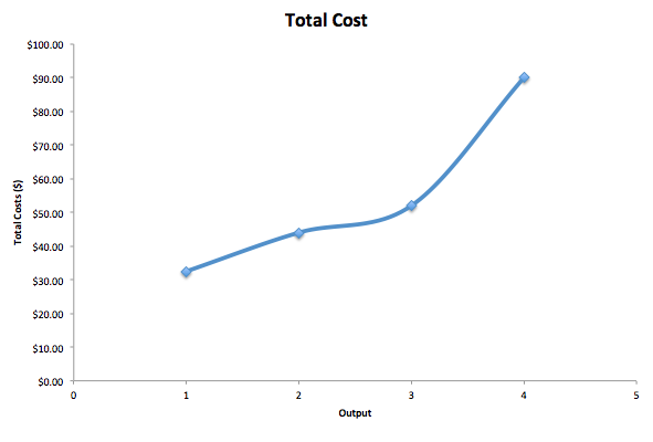
A cost function is a mathematical equation that shows the cost of producing different levels of output. Table 1 gives an example, which shows the cost of producing different quantities of widgets.

Table 1. Cost Function for Producing Widgets
Q	1	2	3	4
Cost	$32.50	$44	$52	$90

What we observe is that the cost increases as the firm produces higher quantities of output. This is pretty intuitive, since producing more output requires greater quantities of inputs, which cost more dollars to acquire.

What is the origin of these cost figures? They come from the production function and the factor payments. Suppose the production function for widgets is as shown in Table 2:

Table 2. Number of Workers and Widgets Produced
Workers (L)	1	2	3	3.25	4.4	5.2	6	7	8	9
Widgets (Q)	0.2	0.4	0.8	1	2	3	3.5	3.8	3.95	4

We can use the information from the production function to determine production costs. What we need to know is how many workers are required to produce any quantity of output. If we flip the order of the rows, we “invert” the production function so it shows $L=g\left(Q\right)$ .

Table 3. Widgets Produced by Workers
Widgets (Q)	0.2	0.4	0.8	1	2	3	3.5	3.8	3.95	4
Workers (L)	1	2	3	3.25	4.4	5.2	6	7	8	9

Now focus on the whole number quantities of output. We’ll eliminate the fractions (or partial widgets) from the table:

Table 4. Number of Widgets Produced
Widgets (Q)	1	2	3	4
Workers (L)	3.25	4.4	5.2	9

Suppose widget workers receive $10 per hour. Multiplying the Workers row by $10 (and eliminating the blanks) gives us the cost of producing different levels of output.

Table 5. Cost of Producing Widgets
Widgets (Q)	1.00	2.00	3.00	4.00
Workers (L)	3.25	4.4	5.2	9
× Wage Rate per hour	$10	$10	$10	$10
= Cost	$32.50	$44.00	$52.00	$90.00

This is same cost function with which we began (shown in Table 1). Figure 2 shows the graph of the cost function.

Upward sloping line showing the total cost curve.

Figure 2.The Total Cost curve for Widgets. This shows cost increasing at an increasing rate as the firm produces more output.

Try It

https://assessments.lumenlearning.co...sessments/7985

Now that we have the basic idea of the cost origins and how they are related to production, let’s drill down into the details, by examining average, marginal, fixed, and variable costs.

Average and Marginal Costs

The cost of producing a firm’s output depends on how much labor and capital the firm uses. A list of the costs involved in producing cars will look very different from the costs involved in producing computer software or haircuts or fast-food meals.

We can measure costs in a variety of ways. Each way provides its own insight into costs. Sometimes firms need to look at their cost per unit of output, not just their total cost. There are two ways to measure per unit costs. The most intuitive way is average cost. Average cost is the cost on average of producing a given quantity. We define average cost as total cost divided by the quantity of output produced.

$AC=TC/Q$

If producing two widgets costs a total of $44, the average cost per widget is

$$44/2=$22$

per widget. The other way of measuring cost per unit is marginal cost. If average cost is the cost of the average unit of output produced, marginal cost is the cost of each individual unit produced. More formally, marginal cost is the cost of producing one more unit (or a few more units) of output. Mathematically, marginal cost is the change in total cost divided by the change in output:

$MC=\Delta TC/\Delta Q$ .

If the cost of the first widget is $32.50 and the cost of two widgets is $44, the marginal cost of the second widget is

$$44-$32.50=$11.50$

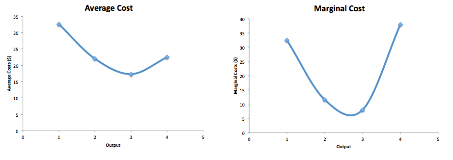
We can see the Widget Cost table redrawn below with average and marginal cost added.

Table 6. Extended Cost Function for Producing Widgets
Q	1	2	3	4
Total Cost	$32.50	$44.00	$52.00	$90.00
Average Cost	$32.50	$22.00	$17.33	$22.50
Marginal Cost	$32.50	$11.50	$8.00	$38.00

Note that the marginal cost of the first unit of output is always the same as total cost. Figures 3a and 3b show the graphs of average and marginal cost respectively. The typical shape of each is a U-shape, with average/marginal cost falling at low levels of output and rising at higher levels of output.

Figure a shows an average cost curve, which starts high, slopes down and then rises slightly. Figure b shows the marginal cost curve, which is a larger u-shape and starts high, the slopes down and back up.

Figure 3. Average and Marginal Cost Curves. Figure 3a shows the average cost of producing widgets based on the data in Table 6. Figure 3b shows the marginal cost of producing widgets. Both average and marginal cost curves typically are U-shaped.

Try It

https://assessments.lumenlearning.co...sessments/7986

https://assessments.lumenlearning.co...sessments/7987

Fixed and Variable Costs

Remember, we explained earlier that fixed inputs are those that cannot be easily adjusted, like a building lease, and variable inputs are those that can be changed easily, like pizza ingredients. We can apply these same terms to costs. Fixed costs are the costs of the fixed inputs. Fixed costs do not change regardless of the level of production, at least not in the short term. Whether you produce a lot or a little, the fixed costs are the same. One example is the rent on a factory or a retail space. Once you sign the lease, the rent is the same regardless of how much you produce, at least until the lease runs out.

Fixed costs can take many other forms: for example, the cost of machinery or equipment to produce the product, research and development costs to develop new products, even an expense like advertising to popularize a brand name. The level of fixed costs varies according to the specific line of business: for instance, manufacturing computer chips requires an expensive factory, but a local moving and hauling business can get by with almost no fixed costs at all if it rents trucks by the day when needed.

Variable costs, on the other hand, are the costs of the variable inputs; they are incurred in the act of producing—the more you produce, the greater the variable cost. Labor is treated as a variable cost, since producing a greater quantity of a good or service typically requires more workers or more work hours. Variable costs would also include raw materials.

As a concrete example of fixed and variable costs, consider a barber shop called “The Clip Joint.” The data for output and costs are shown in Table 7. The fixed costs of operating the barber shop, including the space and equipment, are $160 per day. The variable costs are the costs of hiring barbers, which in our example is $80 per barber each day. The first two columns of the table show the quantity of haircuts the barbershop can produce as it hires additional barbers. The third column shows the fixed costs, which do not change regardless of the level of production. The fourth column shows the variable costs at each level of output. These are calculated by taking the amount of labor hired and multiplying by the wage. For example, two barbers cost: 2 × $80 = $160. Adding together the fixed costs in the third column and the variable costs in the fourth column produces the total costs in the fifth column. So, for example, with two barbers the total cost is: $160 + $160 = $320.

Table 7. Output and Total Costs
Labor	Quantity	Fixed Cost	Variable Cost	Total Cost
1	16	$160	$80	$240
2	40	$160	$160	$320
3	60	$160	$240	$400
4	72	$160	$320	$480
5	80	$160	$400	$560
6	84	$160	$480	$640
7	82	$160	$560	$720

The relationship between the quantity of output being produced and the cost of producing that output is shown graphically in the Figure 4. The fixed costs are always shown as the vertical intercept of the total cost curve; that is, they are the costs incurred when output is zero so there are no variable costs. You can see from the graph that once production starts, total costs and variable costs rise. While variable costs may initially increase at a decreasing rate, at some point they begin increasing at an increasing rate. This is caused by diminishing marginal returns, which is easiest to see with an example. As the number of barbers increases from zero to one in the table, output increases from 0 to 16 for a marginal gain of 16; as the number rises from one to two barbers, output increases from 16 to 40, a marginal gain of 24. From that point on, though, the marginal gain in output diminishes as each additional barber is added.

The graph shows how costs increase with output. It shows a cost curve that starts a 0 with a total cost around $180, then as output increases, so does the total cost, until at an output of 90, the cost is $650.

Figure 4. “The Clip Joint” Total Costs. At zero production, the fixed costs of $160 are still present. As production increases, variable costs are added to fixed costs, and the total cost is the sum of the two.

For example, as the number of barbers rises from two to three, the marginal output gain is only 20; and as the number rises from three to four, the marginal gain is only 12. To understand the reason behind this pattern, consider that a one-man barber shop is a very busy operation. The single barber needs to do everything: say hello to people entering, answer the phone, cut hair, sweep up, and run the cash register. A second barber reduces the level of disruption from jumping back and forth between these tasks, and allows a greater division of labor and specialization. The result can be greater increasing marginal returns. However, as other barbers are added, the advantage of each additional barber is less, since the specialization of labor can only go so far. The addition of a sixth or seventh or eighth barber just to greet people at the door will have less impact than the second one did. This is the pattern of diminishing marginal returns. At some point, you may even see negative returns as the additional barbers begin bumping elbows and getting in each other’s way. In this case, the addition of still more barbers would actually cause output to decrease, as shown in the last row of Table 1. As a result, the total costs of production will begin to rise more rapidly as output increases.

This pattern of diminishing marginal returns is common in production. As another example, consider the problem of irrigating a crop on a farmer’s field. The plot of land is the fixed factor of production, while the water that can be added to the land is the key variable cost. As the farmer adds water to the land, output increases. But adding more and more water brings smaller and smaller increases in output, until at some point the water floods the field and actually reduces output. Diminishing marginal returns occur because, at a given level of fixed costs, each additional input contributes less and less to overall production.

Try It

https://assessments.lumenlearning.co...sessments/7988

Watch It

Watch this clip to review and assess your ability to identify the variable, fixed, total, and marginal costs.

A link to an interactive elements can be found at the bottom of this page.

Try It

These questions allow you to get as much practice as you need, as you can click the link at the top of the first question (“Try another version of these questions”) to get a new set of questions. Practice until you feel comfortable doing the questions.

[ohm_question sameseed=1]155067-155068-155069[/ohm_question]

Learning Objectives

[glossary-page][glossary-term]Factor payments: [/glossary-term]
[glossary-definition]what the firm pays for the use of the factors of production-includes raw materials, rent, wages and salaries, interest and dividends, and profit for entrepreneurship.[/glossary-definition][glossary-term]fixed cost:[/glossary-term]
[glossary-definition]cost of the fixed inputs; expenditure that a firm must make before production starts and that does not change regardless of the production level[/glossary-definition][glossary-term]marginal cost:[/glossary-term]
[glossary-definition]the additional cost of producing one more unit; mathematically, $MC=\Delta TC/\Delta Q$ .[/glossary-definition][glossary-term]total cost:[/glossary-term]
[glossary-definition]the sum of fixed and variable costs of production[/glossary-definition][glossary-term]variable cost:[/glossary-term]
[glossary-definition]cost of production that increases with the quantity produced; the cost of the variable inputs[/glossary-definition]
[/glossary-page]

Contributors and Attributions

Modification, adaptation, and original content. Provided by: Lumen Learning. License: CC BY: Attribution

Costs in the Short Run. Provided by: OpenStax College. Located at: https://cnx.org/contents/XAl2LLVA@7.23:kDmsPrPJ@13/Costs-in-the-Short-Run. License: CC BY: Attribution. License Terms: Download for free at http://cnx.org/contents/bc498e1f-efe...569ad09a82@4.4

Costs of Production. Provided by: ACDC Leadership. Located at: https://www.youtube.com/watch?v=ucJBO9UTmwo. License: Other. License Terms: Standard YouTube License