
10.14: Calculating Profits and Losses
- Page ID
- 48418
Learning Objectives
- Describe a firm’s profit margin
- Use the average cost curve to calculate and analyze a firm’s profits and losses
- Identify and explain the firm’s break-even point
Profits and Losses with the Average Cost Curve
Does maximizing profit (producing where MR = MC) imply an actual economic profit? The answer depends on firm’s profit margin (or average profit), which is the relationship between price and average total cost. If the price that a firm charges is higher than its average cost of production for that quantity produced, then the firm’s profit margin is positive and it is earning economic profits. Conversely, if the price that a firm charges is lower than its average cost of production, the firm’s profit margin is negative and it is suffering an economic loss. You might think that, in this situation, the farmer may want to shut down immediately. Remember, however, that the firm has already paid for fixed costs, such as equipment, so it may make sense to continue to produce and incur a loss. Figure 1 illustrates three situations: (a) where at the profit maximizing quantity of output (where P = MC), price is greater than average cost, (b) where at the profit maximizing quantity of output (where P = MC), price equals average cost, and (c) where at the profit maximizing quantity of output (where P = MC), price is less than average cost.
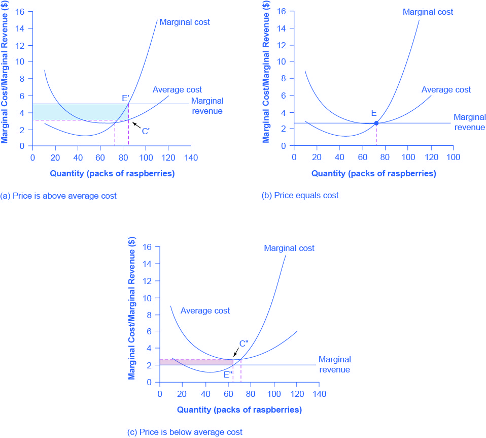
First consider a situation where the price is equal to $5 for a pack of frozen raspberries. The rule for a profit-maximizing perfectly competitive firm is to produce the level of output where Price= MR = MC, so the raspberry farmer will produce a quantity of approximately 85, which is labeled as E’ in Figure 1(a). The firm’s average cost of production is labeled C’. Thus, the firm’s profit margin is the distance between E’ and C’, and it is positive. The firm is making money, but how much? Remember that the area of a rectangle is equal to its base multiplied by its height. The farm’s total revenue at this price will be shown by the rectangle from the origin over to a quantity of 85 packs (the base) up to point E’ (the height), over to the price of $5, and back to the origin. The average cost of producing 85 packs is shown by point C’ or about $3.50. Total costs will be the quantity of 85 times the average cost of $3.50, which is shown by the area of the rectangle from the origin to a quantity of 90, up to point C, over to the vertical axis and down to the origin. The difference between total revenues and total costs is profits. Thus, profits will be the blue shaded rectangle on top.
We calculate this as:
Or, we can calculate it as:
Now consider Figure 1(b), where the price has fallen to $2.75 for a pack of frozen raspberries. Again, the perfectly competitive firm will choose the level of output where Price = MR = MC, but in this case, the quantity produced will be 75. At this price and output level, where the marginal cost curve is crossing the average cost curve, the price the firm receives is exactly equal to its average cost of production. We call this the break-evenpoint, since the profit margin is zero.
The farm’s total revenue at this price will be shown by the large shaded rectangle from the origin over to a quantity of 75 packs (the base) up to point E (the height), over to the price of $2.75, and back to the origin. The height of the average cost curve at Q = 75, i.e. point E, shows the average cost of producing this quantity. Total costs will be the quantity of 75 times the average cost of $2.75, which is shown by the area of the rectangle from the origin to a quantity of 75, up to point E, over to the vertical axis and down to the origin. It should be clear that the rectangles for total revenue and total cost are the same. Thus, the firm is making zero profit. The calculations are as follows:
Or, we can calculate it as:
In Figure 1(c), the market price has fallen still further to $2.00 for a pack of frozen raspberries. At this price, marginal revenue intersects marginal cost at a quantity of 65. The farm’s total revenue at this price will be shown by the large shaded rectangle from the origin over to a quantity of 65 packs (the base) up to point E” (the height), over to the price of $2, and back to the origin. The average cost of producing 65 packs is shown by Point C” which shows the average cost of producing 50 packs is about $2.73. Since the price is less than average cost, the firm’s profit margin is negative. Total costs will be the quantity of 65 times the average cost of $2.73, which the area of the rectangle from the origin to a quantity of 50, up to point C”, over to the vertical axis and down to the origin shows. It should be clear from examining the two rectangles that total revenue is less than total cost. Thus, the firm is losing money and the loss (or negative profit) will be the rose-shaded rectangle.
The calculations are:
Or:
If the market price that a perfectly competitive firm receives leads it to produce at a quantity where the price is greater than average cost, the firm will earn profits. If the price the firm receives causes it to produce at a quantity where price equals average cost, which occurs at the minimum point of the AC curve, then the firm earns zero profits. Finally, if the price the firm receives leads it to produce at a quantity where the price is less than average cost, the firm will earn losses. Table 1 summarizes this.
Try It
https://assessments.lumenlearning.co...sessments/8087
| Table 1. Profit and Average Total Cost | |
|---|---|
| If… | Then… |
| Price > ATC | Firm earns an economic profit |
| Price = ATC | Firm earns zero economic profit |
| Price < ATC | Firm earns a loss |
Which intersection should a firm choose?
At a price of $2, MR intersects MC at two points: Q = 20 and Q = 65. It never makes sense for a firm to choose a level of output on the downward sloping part of the MC curve, because the profit is lower (the loss is bigger). Thus, the correct choice of output is Q = 65.
Watch It
Watch this video for more practice solving for the profit-maximizing point and finding total revenue using a table.
Try It
Play the simulation below multiple times to practice applying these concepts and to see how different choices lead to different outcomes.
Try It
These questions allow you to get as much practice as you need, as you can click the link at the top of the first question (“Try another version of these questions”) to get a new set of questions. Practice until you feel comfortable doing the questions.
[ohm_question]155101-155102-155103-155094[/ohm_question]
Glossary
[glossary-page][glossary-term]break-even point:[/glossary-term]
[glossary-definition] the level of output where price just equals average total cost, so profit is zero[/glossary-definition][glossary-term]profit margin: [/glossary-term]
[glossary-definition]at any given quantity of output, the difference between price and average total cost; also known as average profit[/glossary-definition][/glossary-page]
Contributors and Attributions
- Maximizing Profit. Authored by: Clark Aldrich for Lumen Learning. License: CC BY: Attribution
- How Perfectly Competitive Firms Make Output Decisions. Authored by: OpenStax College. Located at: https://cnx.org/contents/vEmOH-_p@4.48:EkZLadKh@7/How-Perfectly-Competitive-Firm. License: CC BY: Attribution. License Terms: Download for free at http://cnx.org/contents/bc498e1f-efe...69ad09a82@4.44
- Maximizing Profit Practice- Micro 3.9. Provided by: ACDC Leadership. Located at: https://www.youtube.com/watch?v=BQvtnjWZ0ig. License: Other. License Terms: Standard YouTube License