
9.6: Economies of Scale
- Page ID
- 48406
Learning Objectives
- Identify economies of scale, diseconomies of scale, and constant returns to scale
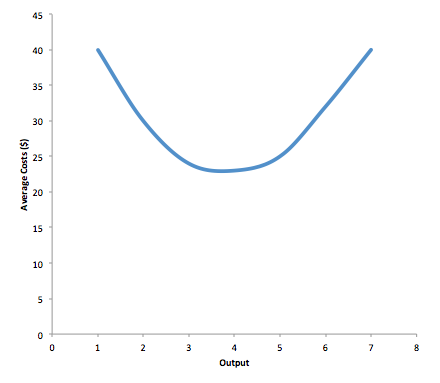
Earlier in this module we saw that in the short run when a firm increases its scale of operation (or its level of output), its average cost of production can decrease or increase. This is illustrated in Figure 1.
What happens to a firm’s average costs when it increases its level of output in the long run? Many industries experience economies of scale. Economies of scale refers to the situation where, as the quantity of output goes up, the cost per unit goes down. This is the idea behind “warehouse stores” like Costco or Walmart. In everyday language: a larger factory can produce at a lower average cost than a smaller factory. Figure 1 illustrates the idea of economies of scale, showing the average cost of producing an alarm clock falling as the quantity of output rises. For a small-sized factory like S, with an output level of 1,000, the average cost of production is $12 per alarm clock. For a medium-sized factory like M, with an output level of 2,000, the average cost of production falls to $8 per alarm clock. For a large factory like L, with an output of 5,000, the average cost of production declines still further to $4 per alarm clock.

The average cost curve in Figure 2 may appear similar to the average cost curve in Figure 1, although it is downward-sloping rather than U-shaped. But there is one major difference. The economies of scale curve is a long-run average cost curve, because it allows all factors of production to change. Short-run average cost curves assume the existence of fixed costs, and only variable costs were allowed to change. In sum, economies of scale refers to a situation where long run average cost decreases as the firm’s output increases.
One prominent example of economies of scale occurs in the chemical industry. Chemical plants have a lot of pipes. The cost of the materials for producing a pipe is related to the circumference of the pipe and its length. However, the volume of chemicals that can flow through a pipe is determined by the cross-section area of the pipe. The calculations in Table 1 show that a pipe which uses twice as much material to make (as shown by the circumference of the pipe doubling) can actually carry four times the volume of chemicals because the cross-section area of the pipe rises by a factor of four (as shown in the Area column).
| Table 1. Comparing Pipes: Economies of Scale in the Chemical Industry | ||
|---|---|---|
| Circumference (2πr) | Area (πr2) | |
| 4-inch pipe | 12.5 inches | 12.5 square inches |
| 8-inch pipe | 25.1 inches | 50.2 square inches |
| 16-inch pipe | 50.2 inches | 201.1 square inches |
A doubling of the cost of producing the pipe allows the chemical firm to process four times as much material. This pattern is a major reason for economies of scale in chemical production, which uses a large quantity of pipes. Of course, economies of scale in a chemical plant are more complex than this simple calculation suggests. But the chemical engineers who design these plants have long used what they call the “six-tenths rule,” a rule of thumb which holds that increasing the quantity produced in a chemical plant by a certain percentage will increase total cost by only six-tenths as much.
Watch It
Watch this video to see an example of economies of scale as applied to making bread.
Shapes of Long-Run Average Cost Curves
While in the short run firms are limited to operating on a single average cost curve (corresponding to the level of fixed costs they have chosen), in the long run when all costs are variable, they can choose to operate on any average cost curve. Thus, the long-run average cost (LRAC) curve is actually based on a group of short-run average cost (SRAC) curves, each of which represents one specific level of fixed costs. More precisely, the long-run average cost curve will be the least expensive average cost curve for any level of output. Figure 3 shows how the long-run average cost curve is built from a group of short-run average cost curves.
Five short-run-average cost curves appear on the diagram. Each SRAC curve represents a different level of fixed costs. For example, you can imagine SRAC1 as a small factory, SRAC2 as a medium factory, SRAC3 as a large factory, and SRAC4 and SRAC5 as very large and ultra-large. Although this diagram shows only five SRAC curves, presumably there are an infinite number of other SRAC curves between the ones that we show. Think of this family of short-run average cost curves as representing different choices for a firm that is planning its level of investment in fixed cost physical capital—knowing that different choices about capital investment in the present will cause it to end up with different short-run average cost curves in the future.

The long-run average cost curve shows the cost of producing each quantity in the long run, when the firm can choose its level of fixed costs and thus choose which short-run average costs it desires. If the firm plans to produce in the long run at an output of Q3, it should make the set of investments that will lead it to locate on SRAC3, which allows producing q3 at the lowest cost. A firm that intends to produce Q3 would be foolish to choose the level of fixed costs at SRAC2 or SRAC4. At SRAC2 the level of fixed costs is too low for producing Q3 at lowest possible cost, and producing q3 would require adding a very high level of variable costs and make the average cost very high. At SRAC4, the level of fixed costs is too high for producing q3 at lowest possible cost, and again average costs would be very high as a result.
The shape of the long-run cost curve, in Figure 3, is fairly common for many industries. The left-hand portion of the long-run average cost curve, where it is downward- sloping from output levels Q1 to Q2 to Q3, illustrates the case of economies of scale. In this portion of the long-run average cost curve, larger scale leads to lower average costs. We illustrated this pattern earlier in Figure 2.
In the middle portion of the long-run average cost curve, the flat portion of the curve around Q3, economies of scale have been exhausted. In this situation, allowing all inputs to expand does not much change the average cost of production. We call this constant returns to scale. In this LRAC curve range, the average cost of production does not change much as scale rises or falls.
How do Economies of Scale Compare to Diminishing Marginal Returns?
The concept of economies of scale, where average costs decline as production expands, might seem to conflict with the idea of diminishing marginal returns, where marginal costs rise as production expands. But diminishing marginal returns refers only to the short-run average cost curve, where one variable input (like labor) is increasing, but other inputs (like capital) are fixed. Economies of scale refers to the long-run average cost curve where all inputs are being allowed to increase together. Thus, it is quite possible and common to have an industry that has both diminishing marginal returns when only one input is allowed to change, and at the same time has increasing or constant economies of scale when all inputs change together to produce a larger-scale operation.
Finally, the right-hand portion of the long-run average cost curve, running from output level Q4 to Q5, shows a situation where, as the level of output and the scale rises, average costs rise as well. This situation is called diseconomies of scale. A firm or a factory can grow so large that it becomes very difficult to manage, resulting in unnecessarily high costs as many layers of management try to communicate with workers and with each other, and as failures to communicate lead to disruptions in the flow of work and materials. Not many overly large factories exist in the real world, because with their very high production costs, they are unable to compete for long against plants with lower average costs of production. However, in some planned economies, like the economy of the old Soviet Union, plants that were so large as to be grossly inefficient were able to continue operating for a long time because government economic planners protected them from competition and ensured that they would not make losses.
Diseconomies of scale can also be present across an entire firm, not just a large factory. The leviathan effect can hit firms that become too large to run efficiently, across the entirety of the enterprise. Firms that shrink their operations are often responding to finding itself in the diseconomies region, thus moving back to a lower average cost at a lower output level.
Learning Objectives
- [glossary-page][glossary-term]constant returns to scale:[/glossary-term]
[glossary-definition]expanding all inputs proportionately does not change the average cost of production[/glossary-definition][glossary-term]economies of scale:[/glossary-term]
[glossary-definition]the long-run average cost of producing output decreases as total output increases[/glossary-definition][glossary-term]diseconomies of scale:[/glossary-term]
[glossary-definition]the long-run average cost of producing output increases as total output increases[/glossary-definition][glossary-term]leviathan effect:[/glossary-term]
[glossary-definition]when a firm gets so large that it operates inefficiently, experiencing diseconomies of scale[/glossary-definition][glossary-term]long-run average cost (LRAC) curve:[/glossary-term]
[glossary-definition]shows the lowest possible average cost of production, allowing all the inputs to production to vary so that the firm is choosing its production technology[/glossary-definition][glossary-term]short-run average cost (SRAC) curve:[/glossary-term]
[glossary-definition]the average total cost curve in the short term; shows the total of the average fixed costs and the average variable costs[/glossary-definition]
[/glossary-page]
Contributors and Attributions
- Modification, adaptation, and original content. Provided by: Lumen Learning. License: CC BY: Attribution
- Economics of Scale. Authored by: OpenStax College. Located at: https://cnx.org/contents/vEmOH-_p@4.48:9SU8XZqL@9/Costs-in-the-Long-Run. License: CC BY: Attribution. License Terms: Download for free at http://cnx.org/contents/bc498e1f-efe...69ad09a82@4.44
- Economies of Scale. Provided by: ACDC Leadership. Located at: https://www.youtube.com/watch?v=JdCgu1sOPDo. License: Other. License Terms: Standard YouTube License