10.7: Equilibrium in the Income-Expenditure Model

Last updated
Save as PDF

Page ID: 47440

$ \newcommand{\vecs}[1]{\overset { \scriptstyle \rightharpoonup} {\mathbf{#1}} } $ $ \newcommand{\vecd}[1]{\overset{-\!-\!\rightharpoonup}{\vphantom{a}\smash {#1}}} $$\newcommand{\id}{\mathrm{id}}$ $ \newcommand{\Span}{\mathrm{span}}$ $ \newcommand{\kernel}{\mathrm{null}\,}$ $ \newcommand{\range}{\mathrm{range}\,}$ $ \newcommand{\RealPart}{\mathrm{Re}}$ $ \newcommand{\ImaginaryPart}{\mathrm{Im}}$ $ \newcommand{\Argument}{\mathrm{Arg}}$ $ \newcommand{\norm}[1]{\| #1 \|}$ $ \newcommand{\inner}[2]{\langle #1, #2 \rangle}$ $ \newcommand{\Span}{\mathrm{span}}$ $\newcommand{\id}{\mathrm{id}}$ $ \newcommand{\Span}{\mathrm{span}}$ $ \newcommand{\kernel}{\mathrm{null}\,}$ $ \newcommand{\range}{\mathrm{range}\,}$ $ \newcommand{\RealPart}{\mathrm{Re}}$ $ \newcommand{\ImaginaryPart}{\mathrm{Im}}$ $ \newcommand{\Argument}{\mathrm{Arg}}$ $ \newcommand{\norm}[1]{\| #1 \|}$ $ \newcommand{\inner}[2]{\langle #1, #2 \rangle}$ $ \newcommand{\Span}{\mathrm{span}}$$\newcommand{\AA}{\unicode[.8,0]{x212B}}$

Learning Objectives

Explain macro equilibrium using the income-expenditure model
Identify macro equilibrium graphically and using tables

In the AD-AS model, we identified the macro equilibrium at the level of GDP where AD=AS. We now have the tools to identify macro equilibrium in the income-expenditure model. Macro equilibrium occurs at the level of GDP where national income equals aggregate expenditure. Let’s find the macro equilibrium in the graphical model.

The Aggregate Expenditure Function

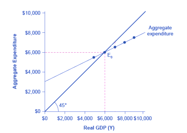
Figure 1 shows the aggregate expenditure function, based on data in Table 1. As we showed in the last section, aggregate expenditure is the sum of consumption expenditure, investment expenditure, government expenditure and net export expenditure.

Table 1. National Income-Aggregate Expenditure Equilibrium
National Income					Aggregate Expenditure
$3,000					$4,620
$4,000					$5,080
$5,000					$5,540
$6,000					$6,000
$7,000					$6,460
$8,000					$6,920
$9,000					$7,380

The graph shows a Keynesian cross diagram with each combination of national income and aggregate expenditure.

Figure 1. A Keynesian Cross Diagram. The combination of the aggregate expenditure line and the income=expenditure line is the Keynesian Cross, that is, the graphical representation of the income-expenditure model. The equilibrium occurs where aggregate expenditure is equal to national income; this occurs where the aggregate expenditure schedule crosses the 45-degree line, at a real GDP of $6,000.

The Income = Expenditure Line

Figure 1 contains two lines that serve as conceptual guideposts to orient the discussion. The first is the aggregate expenditure line that we’ve already discussed. The second conceptual line on the Keynesian cross diagram is the line showing where national income = aggregate expenditure. This line is mathematically the 45-degree line, which starts at the origin and reaches up and to the right. A line that stretches up at a 45-degree angle represents the set of points (1,1), (2,2), (3,3) and so on, where the measurement on the vertical axis is equal to the measurement on the horizontal axis. Thus in this diagram, the 45-degree line shows the set of points where the level of aggregate expenditure in the economy, measured on the vertical axis, is equal to the level of output or national income in the economy, measured by GDP on the horizontal axis. In short, this is our equilibrium condition. The combination of the aggregate expenditure line and the income=expenditure line (i.e. the 45 degree line) is the Keynesian Cross.

Try It

https://assessments.lumenlearning.co...sessments/7571

Where Equilibrium Occurs

Macro equilibrium occurs at the level of GDP where where the aggregate expenditure line crosses the 45-degree line (which shows all points where AE = Y). It is the only point on the aggregate expenditure line where the total quantity of goods and services being purchased (AD) equals the total quantity of goods and services being produced (AS). In Figure 1, this point of equilibrium (E₀) happens at 6,000, which can also be read off Table 1.

The meaning of “equilibrium” remains the same; that is, equilibrium is a point of balance where no incentive exists to shift away from that outcome. To understand why the point of intersection between the aggregate expenditure function and the 45-degree line is a macroeconomic equilibrium, consider what would happen if an economy found itself to the right of the equilibrium point E, say point H in Figure 2, where output is higher than the equilibrium. At point H, the level of aggregate expenditure is below the 45-degree line, so that the level of aggregate expenditure in the economy is less than the level of output. As a result, at point H, output is piling up unsold—not a sustainable state of affairs. Firms will respond by decreasing their level of production and GDP will fall.

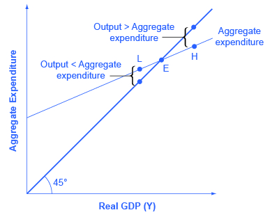
The graph shows the only point at which there can be equilibrium in the Keynesian cross diagram.

Figure 2. Equilibrium in the Keynesian Cross Diagram. If output was above the equilibrium level, at H, then the real output is greater than the aggregate expenditure in the economy. If output was below the equilibrium level at L, then aggregate expenditure would be greater than output. Only point E can be at equilibrium, where output, or national income and aggregate expenditure, are equal. The equilibrium (E) must lie on the 45-degree line, which is the set of points where national income and aggregate expenditure are equal.

Conversely, consider the situation where the level of output is at point L—where real output is lower than the equilibrium. In that case, the level of aggregate demand in the economy is above the 45-degree line, indicating that the level of aggregate expenditure in the economy is greater than the level of output. When the level of aggregate demand has emptied the store shelves, it cannot be sustained, either. Firms will respond by increasing their level of production and GDP will rise. Thus, the equilibrium must be the point where the amount produced and the amount spent are in balance, at the intersection of the aggregate expenditure function and the 45-degree line.

Try It

https://assessments.lumenlearning.co...sessments/7572

Try It

This exercise is designed to show you how to find a new equilibrium in the income-expenditure model following a change in aggregate expenditure.

An interactive or media element has been excluded from this version of the text. You can view it online here: http://pb.libretexts.org/mlum/?p=445

Glossary

[glossary-page][glossary-term]Aggregate Expenditure Function:[/glossary-term][glossary-definition]graphical relationship between national income and aggregate expenditure, which is defined as consumption plus investment plus government spending plus net exports[/glossary-definition][glossary-term]Aggregate Expenditure Schedule:[/glossary-term][glossary-definition]aggregate expenditure function expressed as a table[/glossary-definition][glossary-term]Consumption Function:[/glossary-term][glossary-definition]graphical relationship between national income and consumption expenditure; algebraically: C = a + MPC*Y, where a is autonomous consumption (the amount of consumption expenditure when Y = 0), MPC is the marginal propensity to consume, and Y is national income[/glossary-definition][glossary-term]Income = Expenditure Line:[/glossary-term]
[glossary-definition]all combinations of national income and aggregate expenditure where national income equals aggregate expenditure; graphically, this is the 45 degree line on the Keynesian Cross diagram (or income-expenditure model)[/glossary-definition][glossary-term]Marginal Propensity to Consume:[/glossary-term][glossary-definition]fraction of any change in income which is spent; algebraically MPC = ΔC/ΔY[/glossary-definition][glossary-term]Marginal Propensity to Save:[/glossary-term][glossary-definition]fraction of any change in income which is saved; algebraically MPS = ΔS/ΔY[/glossary-definition]
[/glossary-page]

Appendix B. Authored by: OpenStax College. Provided by: Rice University. Located at: http://cnx.org/contents/4061c832-098e-4b3c-a1d9-7eb593a2cb31@10.49:2/Macroeconomics. License: CC BY: Attribution. License Terms: Download for free at http://cnx.org/donate/download/4061c...cb31@10.49/pdf
Modification, adaptation, and original content. Provided by: Lumen Learning. License: CC BY: Attribution