Introduction to the Aggregate Demand-Aggregate Supply Model
The economic history of the United States is cyclical in nature with recessions and expansions. Some of these fluctuations are severe, such as the economic downturn experienced during Great Depression of the 1930’s which lasted for a decade. Why does the economy grow at different rates in different years? What are the causes of the cyclical behavior of the economy?
A key part of macroeconomics is the use of models to analyze macro issues and problems. How is the rate of economic growth connected to changes in the unemployment rate? Is there a reason why unemployment and inflation seem to move in opposite directions: lower unemployment and higher inflation from 1997 to 2000, higher unemployment and lower inflation in the early 2000s, lower unemployment and higher inflation in the mid-2000s, and then higher unemployment and lower inflation in 2009? Why did the current account deficit rise so high, but then decline in 2009?
To analyze questions like these, we must move beyond discussing macroeconomic issues one at a time, and begin building economic models that will capture the relationships and interconnections between them. This module introduces the macroeconomic model of aggregate demand and aggregate supply, how the two interact to reach a macroeconomic equilibrium, and how shifts in aggregate demand or aggregate supply will affect that equilibrium. This section also relates the model of aggregate demand and aggregate supply to the three goals of economic policy (economic growth, stable prices (low inflation), and full employment), and provides a framework for thinking about many of the connections and tradeoffs between these goals. This model will aid us in understanding why economies expand and contract over time.
A simple version of the AD-AS graph is shown in Figure 1. The horizontal x-axis shows the real output, or GDP of the macroeconomy. The vertical y-axis shows the price level.
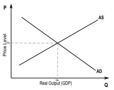
Figure 1. Aggregate Demand-Aggregate Supply Model, showing equilibrium at Pe & Qe.
Watch It
This video provides a nice overview of the key concepts surrounding the aggregate demand-aggregate supply model that we will cover in the next few sections. Watch it carefully so that you have a context for the explanations, diagrams and examples that follow.
A link to an interactive elements can be found at the bottom of this page.
FROM HOUSING BUBBLE TO HOUSING BUST
The United States experienced rising home ownership rates for most of the last two decades. Between 1990 and 2006, the U.S. housing market grew. Homeownership rates grew from 64% to a high of over 69% between 2004 and 2005. For many people, this was a period in which they could either buy first homes or buy a larger and more expensive home. During this time mortgage values tripled. Housing became more accessible to Americans and was considered to be a safe financial investment. Figure 2 shows how new single family home sales peaked in 2005 at 107,000 units.
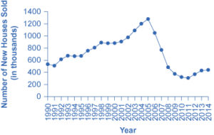
Figure 2. New Single Family Houses Sold. From the early 1990s up through 2005, the number of new single family houses sold rose steadily. In 2006, the number dropped dramatically and this dramatic decline continued through 2011. In 2012, the number sold rose a bit over previous years, but it was still lower than the number of new houses sold in 1990. (Source: U.S. Census Bureau)
The housing bubble began to show signs of bursting in 2005, as delinquency and late payments began to grow and an oversupply of new homes on the market became apparent. Dropping home values contributed to a decrease in the overall wealth of the household sector and caused homeowners to pull back on spending. Several mortgage lenders were forced to file for bankruptcy because homeowners were not making their payments, and by 2008 the problem had spread throughout the financial markets. Lenders clamped down on credit and the housing bubble burst. Financial markets were now in crisis and unable or unwilling to even extend credit to credit-worthy customers.

Figure 3. At the peak of the housing bubble, many people across the country were able to secure the loans necessary to build new houses. (Credit: modification of work by Tim Pierce/Flickr Creative Commons)
The housing bubble and the crisis in the financial markets were major contributors to the Great Recession that led to unemployment rates over 10% and falling GDP. We can show this using AD-AS, but first we need to learn more about the model. While the United States is still recovering from the impact of the Great Recession, it has made substantial progress in restoring financial market stability through the implementation of aggressive fiscal and monetary policy.
Learning Objectives
[glossary-page][glossary-term]aggregate demand/aggregate supply model: [/glossary-term][glossary-definition]a model that shows what determines real GDP and the aggregate price level through the interaction between total spending on domestic goods and services (i.e aggregate demand) and total production by businesses (i.e. aggregate supply)[/glossary-definition][/glossary-page]
