6.8: Cell Format

Last updated
Save as PDF

Page ID: 46509

\( \newcommand{\vecs}[1]{\overset { \scriptstyle \rightharpoonup} {\mathbf{#1}} } \) \( \newcommand{\vecd}[1]{\overset{-\!-\!\rightharpoonup}{\vphantom{a}\smash {#1}}} \)\(\newcommand{\id}{\mathrm{id}}\) \( \newcommand{\Span}{\mathrm{span}}\) \( \newcommand{\kernel}{\mathrm{null}\,}\) \( \newcommand{\range}{\mathrm{range}\,}\) \( \newcommand{\RealPart}{\mathrm{Re}}\) \( \newcommand{\ImaginaryPart}{\mathrm{Im}}\) \( \newcommand{\Argument}{\mathrm{Arg}}\) \( \newcommand{\norm}[1]{\| #1 \|}\) \( \newcommand{\inner}[2]{\langle #1, #2 \rangle}\) \( \newcommand{\Span}{\mathrm{span}}\) \(\newcommand{\id}{\mathrm{id}}\) \( \newcommand{\Span}{\mathrm{span}}\) \( \newcommand{\kernel}{\mathrm{null}\,}\) \( \newcommand{\range}{\mathrm{range}\,}\) \( \newcommand{\RealPart}{\mathrm{Re}}\) \( \newcommand{\ImaginaryPart}{\mathrm{Im}}\) \( \newcommand{\Argument}{\mathrm{Arg}}\) \( \newcommand{\norm}[1]{\| #1 \|}\) \( \newcommand{\inner}[2]{\langle #1, #2 \rangle}\) \( \newcommand{\Span}{\mathrm{span}}\)\(\newcommand{\AA}{\unicode[.8,0]{x212B}}\)

Learning Objectives

Change cell format.

As mentioned previously, Excel will default to certain styles when you create a new worksheet. In particular, this includes the way that numbers are displayed and whether or not commas are automatically included. In this section, we will take a look at changing these defaults.

When you type numbers into an Excel workbook, it will often default to a specific format. For example, if you type “12/15/17,” Excel will convert this to read “12/15/2017,” assuming you were entering month, day, and abbreviated year. Similarly, “3/4” will display at “4-Mar,” the fourth day of March. However, it is possible that you may have been entering fractions, so “3/4” was meant to indicate three-quarters instead.

If this is the case, you will need to format your cells to properly display the information you are entering. When possible, consider formatting your cells before you enter the data. Otherwise, Excel may convert some of the entries and you will need to re-enter that information.

Method 1

A blank Microsoft Excel sheet is open. There are three numbers each representing a different aspect of the sheet. The first number is green and shows a box which is highlighting a section of cells that have been selected. The second number is orange and next to it as an arrow that points to the format dropdown menu. The third number is pink and has an arrow next to it pointing at the format cells feature in the format dropdown menu.

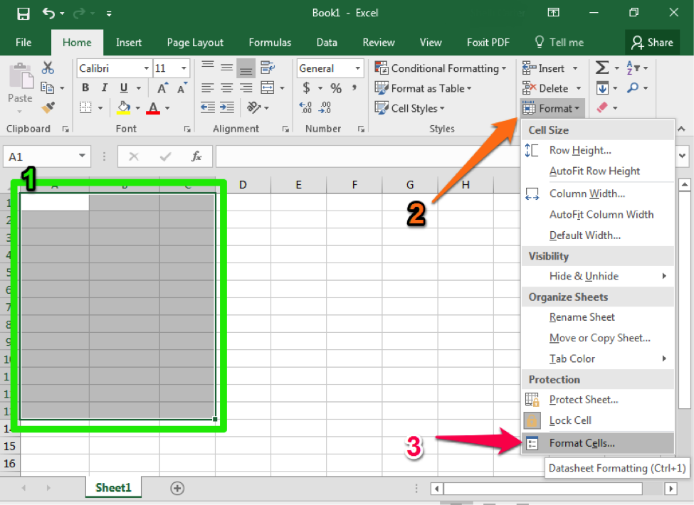
Begin by highlighting the cells you plan to use.
Select the Format dropdown from the Cells group of the ribbon.
Select the Format cells option at the bottom of the dropdown menu.

Practice question

https://assessments.lumenlearning.co...essments/18626

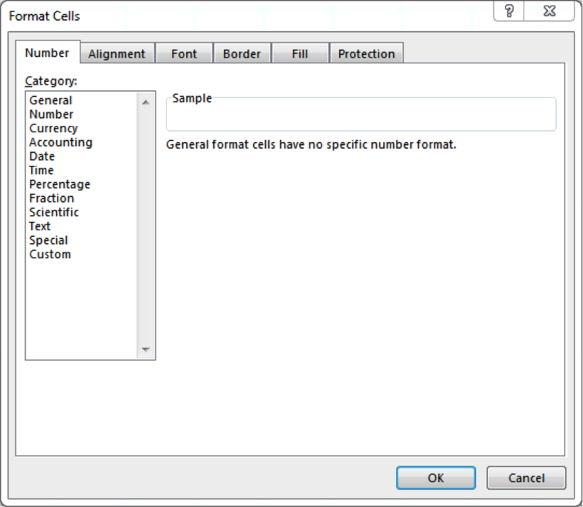
There are several available format options for cells in Excel. When you select one, Excel will provide you with a description and examples of how the information will display in the cells.

Practice question

https://assessments.lumenlearning.co...essments/18627

Method 2

You can perform the same actions using the “Number” group in the ribbon. In this case, you simply select the cell format you wish to apply using the dropdown menu.

A blank Microsoft Excel sheet is open. There is a green arrow pointing at a green box showing where the number group option is.

Contributors and Attributions

Cell Format. Authored by: Shelli Carter. Provided by: Lumen Learning. License: CC BY: Attribution