10.4: Labor Rate Variance

Last updated
Save as PDF

Page ID: 45941

$ \newcommand{\vecs}[1]{\overset { \scriptstyle \rightharpoonup} {\mathbf{#1}} } $ $ \newcommand{\vecd}[1]{\overset{-\!-\!\rightharpoonup}{\vphantom{a}\smash {#1}}} $$\newcommand{\id}{\mathrm{id}}$ $ \newcommand{\Span}{\mathrm{span}}$ $ \newcommand{\kernel}{\mathrm{null}\,}$ $ \newcommand{\range}{\mathrm{range}\,}$ $ \newcommand{\RealPart}{\mathrm{Re}}$ $ \newcommand{\ImaginaryPart}{\mathrm{Im}}$ $ \newcommand{\Argument}{\mathrm{Arg}}$ $ \newcommand{\norm}[1]{\| #1 \|}$ $ \newcommand{\inner}[2]{\langle #1, #2 \rangle}$ $ \newcommand{\Span}{\mathrm{span}}$ $\newcommand{\id}{\mathrm{id}}$ $ \newcommand{\Span}{\mathrm{span}}$ $ \newcommand{\kernel}{\mathrm{null}\,}$ $ \newcommand{\range}{\mathrm{range}\,}$ $ \newcommand{\RealPart}{\mathrm{Re}}$ $ \newcommand{\ImaginaryPart}{\mathrm{Im}}$ $ \newcommand{\Argument}{\mathrm{Arg}}$ $ \newcommand{\norm}[1]{\| #1 \|}$ $ \newcommand{\inner}[2]{\langle #1, #2 \rangle}$ $ \newcommand{\Span}{\mathrm{span}}$$\newcommand{\AA}{\unicode[.8,0]{x212B}}$

Learning Outcomes

Analyze the variance between expected labor cost and actual labor costs

So Mary needs to figure out her labor variance with the changes in staffing and wage rate. She is hopeful that Jake will be able to step up to the plate and there won’t be any changes in the .5 hours per pair of shoes that she initially budgeted. Here is a quick review of what is included in direct labor!

So here is Mary’s new direct labor costs:

	Total
Required Production in Pairs	2050
Direct labor hours-pair	0.5
Total direct labor hours needed	1025
Direct labor cost per hour	$22
Total direct labor cost	$22,550

So going back to our chart:

Spending Variance flows into Labor Rate Variance, Actual Hours of Input at Standard Rate, and Labor Efficiency Variance. Labor Rate Variance flows into Actual Hours of Input at Actual Rate. Labor Efficiency Variance flows into Standard Hours Allowed for Actual Output, at Standard Rate.

Actual hours of input at actual rate= 1025 × $22 ƒ= $22,550

Standard hours of input allowed for actual output at standard rate = 1025 × $20 = $20,000

There is a labor rate variance of $2,550 unfavorable.

So Mary takes this information to her boss, explaining that she was unable to find a qualified employee at the old rate. She also wanted to make sure her staff were happy employees, so she needed to bring them all up to that rate as well. It didn’t seem fair to have the new guy making more than her faithful staff. Good management can keep good staff. Mary made a great decision! The decisions we make as managers, may be difficult. Sometimes budgets need to be adjusted, or pricing needs to be changed to continue.

It is always important, as you are starting to see, to look at all options as we work through management decisions. Are we using good materials? Is there more efficient piece of equipment? Do we have properly trained and happy staff members? Let’s continue our discussions surrounding labor rates and hours.

So Jake started work, and it isn’t going as well as expected. The change in staffing has had challenges. The time it takes to make a pair of shoes has gone from .5 to .6 hours. Mary hopes it will better as the team works together, but right now, she needs to reevaluate her labor budget and get the information to her boss.

Here is what the actual looks like now:

	Total
Required Production in Pairs	2050
Direct labor hours-pair	0.6
Total direct labor hours needed	1230
Direct labor cost per hour	$22
Total direct labor cost	$27,060

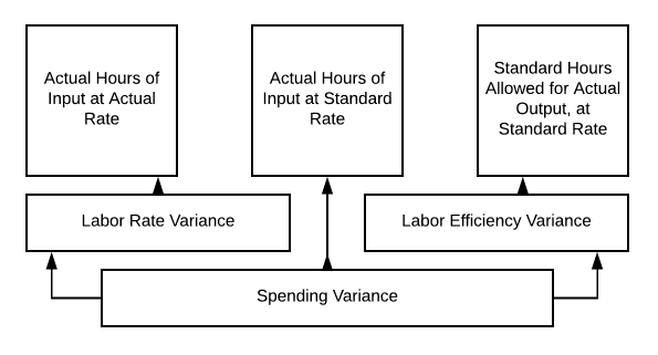
So if we go back to our chart on 10.3, we can calculate our labor variance:

Actual Hours of Input at Actual Rate = 1230 × $22= $27,060
Actual Hours of Input at Standard Rate = 1230 × $20= $24,600
Standard Hours Allowed for Actual Output at Standard Rate = 1025 × $20 = $20,500

So our labor rate variance is $27,060 − $24,600 = $2,460 unfavorable

Actual Hours of Input at Standard Rate = 1230 × $20= $24,600
Standard Hours Allowed for Actual Output at Standard Rate = 1025 × $20= $20,500

So our labor efficiency variance is $24,600 − $20,500= $4,100 unfavorable

Our Spending Variance is the sum of those two numbers, so $6,560 unfavorable ($27,060 − $20,500).

Mary is not excited about taking this information to her boss, but what can she do?

So as we discussed, we can analyze the variance for labor efficiency by using the standard cost variance analysis chart on 10.3.

Mary’s new hire isn’t doing as well as expected, but what if the opposite had happened? What if adding Jake to the team has speeded up the production process and now it was only taking .4 hours to produce a pair of shoes? Let’s examine this situation further.

Even with a higher direct labor cost per hour, our total direct labor cost went down! Let’s take that apart.

Actual Hours of Input at Actual Rate = 820 × $22= $18,040
Actual Hours of Input at Standard Rate = 820 × $20= $16,040
Standard Hours Allowed for Actual Output at Standard Rate = 1025 × $20= $20,500 (our original budget)

So now, our labor rate Variance = $18,040 − $16,040= $2000 unfavorable

(NOTE: We are still paying more per hour than budgeted)

Our labor efficiency variance = $16,040 − $20,500 = $4,460 favorable

And our overall spending variance = $2,460 favorable

We are still spending less on labor, even at a higher rate per hour, so our overall variance is favorable. Now Mary is a happy production manager!

Practice Questions

https://assessments.lumenlearning.co...sessments/9657

Labor Rate Variance. Authored by: Freedom Learning Group. Provided by: Lumen Learning. License: CC BY: Attribution