4.3: Alternative Patterns for Calculating Depreciation

Last updated
Save as PDF

Page ID: 51340

$ \newcommand{\vecs}[1]{\overset { \scriptstyle \rightharpoonup} {\mathbf{#1}} } $ $ \newcommand{\vecd}[1]{\overset{-\!-\!\rightharpoonup}{\vphantom{a}\smash {#1}}} $$\newcommand{\id}{\mathrm{id}}$ $ \newcommand{\Span}{\mathrm{span}}$ $ \newcommand{\kernel}{\mathrm{null}\,}$ $ \newcommand{\range}{\mathrm{range}\,}$ $ \newcommand{\RealPart}{\mathrm{Re}}$ $ \newcommand{\ImaginaryPart}{\mathrm{Im}}$ $ \newcommand{\Argument}{\mathrm{Arg}}$ $ \newcommand{\norm}[1]{\| #1 \|}$ $ \newcommand{\inner}[2]{\langle #1, #2 \rangle}$ $ \newcommand{\Span}{\mathrm{span}}$ $\newcommand{\id}{\mathrm{id}}$ $ \newcommand{\Span}{\mathrm{span}}$ $ \newcommand{\kernel}{\mathrm{null}\,}$ $ \newcommand{\range}{\mathrm{range}\,}$ $ \newcommand{\RealPart}{\mathrm{Re}}$ $ \newcommand{\ImaginaryPart}{\mathrm{Im}}$ $ \newcommand{\Argument}{\mathrm{Arg}}$ $ \newcommand{\norm}[1]{\| #1 \|}$ $ \newcommand{\inner}[2]{\langle #1, #2 \rangle}$ $ \newcommand{\Span}{\mathrm{span}}$$\newcommand{\AA}{\unicode[.8,0]{x212B}}$

Learning Objectives

At the end of this section, students should be able to meet the following objectives:

Explain the justification for accelerated methods of depreciation.
Compute depreciation expense using the double-declining balance method.
Realize that the overall impact on net income is not affected by a particular cost allocation pattern.
Describe the units-of-production method, including its advantages and disadvantages.

Question: Straight-line depreciation certainly qualifies as systematic and rational. The same amount of cost is assigned to expense during each period of use. Because no specific method is required by U.S. GAAP, do companies ever use alternative approaches to create other allocation patterns for depreciation? If so, how are these additional methods justified?

Answer: The most common alternative to the straight-line method is accelerated depreciation, which records a larger expense in the initial years of an asset’s service. The primary rationale for this pattern is that property and equipment often produce higher revenues earlier in their lives because they are newer. The matching principle would suggest that recognizing more depreciation in these periods is appropriate to better align the expense with the revenues earned.

A second justification for accelerated depreciation is that some types of property and equipment lose value more quickly in their first few years than they do in later years. Automobiles and other vehicles are a typical example of this pattern. Recording a greater expense initially is said to better reflect reality.

Over the decades, a number of equations have been invented to mathematically create an accelerated depreciation pattern, high expense at first with subsequent cost allocations falling throughout the life of the property. The most common is the double-declining balance method (DDB). When using DDB, annual depreciation is determined by multiplying the book value of the asset times two divided by the expected years of life. As book value drops, annual expense drops. This formula has no internal logic except that it creates the desired pattern, an expense that is higher in the first years of operation and less after that. Although residual value is not utilized in this computation, the final amount of depreciation recognized must be manipulated to arrive at this proper ending balance.

Depreciation for the building bought above for $600,000 with an expected five-year life and a residual value of $30,000 is calculated as follows if DDB is applied.

(cost – accumulated depreciation) × 2/expected life = depreciation expense for period

Year One:

($600,000 – $0) = $600,000 × 2/5 = $240,000 depreciation expense

Year Two:

($600,000 – $240,000) = $360,000 × 2/5 = $144,000 depreciation expense note using the depreciation from year 1 as accumulated depreciation

Year Three:

($600,000 – $384,000) = $216,000 × 2/5 = $86,400 depreciation expense note using the depreciation from year 1 and 2 as accumulated depreciation

Year Four:

($600,000 – $470,400) = $129,600 × 2/5 = $51,840 depreciation expense

Year Five:

($600,000 – $522,240) = $77,760,

so depreciation for Year Five must be set at $47,760 to arrive at the expected residual value of $30,000. This final expense is always the amount needed to arrive at the expected residual value.

Note that the desired expense pattern has resulted. The expense starts at $240,000 and becomes smaller (declines) in each subsequent period.

Figure 4.3 Building Acquisition and Double-Declining Balance Depreciation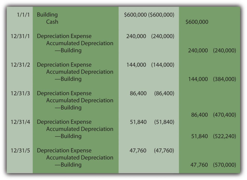 Building recorded like usual. Depreciation expense is 240000 for year 1, 144000 for year 2, 86400 for year three, 51840 for year 4 and 47760 for year 5 - for each year the journal entry is a debit to depreciation expense and credit to accumulated depreciation - a contra asset account. Total depreciation recorded over 5 years is 570000

So while both straight line and double declining balance methods end up with the same total depreciation over 5 years – the amount of depreciation recorded each year is different. Double declining balance records more depreciation and thus will have lower net income in the early years while straight line will have lower net income in the later years.

Check Yourself

If Downtown Company purchases a machine for $120,000 with a useful life of 7 years and an estimated residual value of $10,000, how much depreciation would be recorded in the second year of its useful life using Double Declining Balance?

A. $24,490

B. $31,428

C. $34,286

D. $28,571

The correct answer is A. For year one the calculation would be 120,000 x 2 / 7 = 34,286. Subtract that accumulated depreciation from 120,000. So (120,000 – 34,286) x 2 / 7 = 24,490.

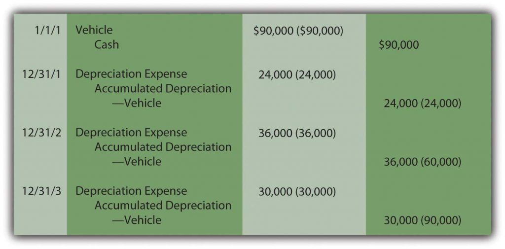
Question: The two methods demonstrated here for establishing a depreciation pattern are based on time, five years to be precise. In most cases, though, it is the physical use of the asset rather than the passage of time that is actually relevant to this process. Use is the action that generates revenues. How is the depreciation of a long-lived tangible asset determined if usage can be measured? For example, assume that a limousine company buys a new vehicle for $90,000 to serve as an addition to its fleet. Company officials expect this limousine to be driven for three hundred thousand miles and then have no residual value. How is depreciation expense determined each period?

Answer: Depreciation does not have to be based on time; it only has to be computed in a systematic and rational manner. Thus, the units-of-production method (UOP) is another alternative that is occasionally encountered. UOP is justified because the periodic expense is matched with the work actually performed. In this illustration, the limousine’s depreciation can be computed using the number of miles driven in a year, an easy figure to determine.

($90,000 less $0)/300,000 miles = $0.30 per mile

Depreciation is recorded at a rate of $0.30 per mile. The depreciable cost basis is allocated evenly over the miles that the vehicle is expected to be driven. UOP is a straight-line method but one that is based on usage (miles driven, in this example) rather than years. Because of the direct connection between the expense allocation and the work performed, UOP is a very appealing approach. It truly mirrors the matching principle. Unfortunately, measuring the physical use of most assets is rarely as easy as with a limousine.

For example, if this vehicle is driven 80,000 miles in Year One, 120,000 miles in Year Two, and 100,000 miles in Year Three, depreciation will be $24,000, $36,000, and $30,000 when the $0.30 per mile rate is applied.

Figure 4.4 Depreciation—Units-of-Production Method

Depreciation expense for year 1 is 24000 and year 2 36000 and year 3 30000. Each year the debit is to depreciation expense and credit to accumulated depreciation

Estimations rarely prove to be precise reflections of reality. This vehicle will not likely be driven exactly three hundred thousand miles. If used for less and then retired, both the cost and accumulated depreciation are removed. A loss is recorded equal to the remaining book value unless some cash or other asset is received. If driven more than the anticipated number of miles, depreciation stops at three hundred thousand miles. At that point, the cost of the asset will have been depreciated completely.

Check Yourself

Which of the following is true with regard to units of production calculation of depreciation?

A. Residual value is ignored in the calculation just like double declining balance.

B. It requires two steps – cost per unit calculation and multiply by units to get depreciation expense.

C. Over the life of an asset the units of production method results in higher total depreciation than double declining balance.

D. Units of production is probably the worst method for matching revenues with expenses.

The answer is B. Residual value is subtracted when calculating the cost per unit and all methods of depreciation must have the same total depreciation amount. Calculating depreciation requires two steps – cost per unit and then multiplying that cost by the number of units for the time period to get the depreciation expense for that time period.

Key Takeaway

Cost allocation patterns for determining depreciation exist beyond just the straight-line method. Accelerated depreciation records more expense in the earlier years of use than in later periods. This pattern is sometimes considered a better matching of expenses with revenues and a closer image of reality. The double-declining balance method is the most common version of accelerated depreciation. Its formula was derived to create the appropriate allocation pattern. The units-of-production method is often used for property and equipment where the quantity of work performed can be easily monitored.