
5.4: Non-Linear Optimization
- Page ID
- 21134

As discussed earlier, most infrastructure management optimization problems are formulated as linear programming problems. However, in some cases, non-linear optimization may be needed. The general form of the non-linear optimization problem is:
\[\text{Minimize or Maximize } f(x) \text{ subject to } g_{i}(x) \leq 0 \text{ and } h_{j}(x)=0\]
Where \(x\) is a vector of decision variables, \(f(x)\) is a non-linear objective function, \(g_i(x)\) and \(h_j(x)\) are sets of constraints which may be linear or non-linear.
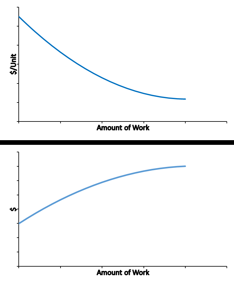
One source of non-linearities is that of scale economies in performing a maintenance or rehabilitation task. This might occur if there are fixed mobilization costs to undertake a task which are then spread over the amount of work. Components such as tanks also have scale economies since their volume grows faster than the (expensive) tank surface as the tank size increases. Figure 5.4.1 illustrates scale economies in two related graphs. In the upper graph, the cost per unit of work declining as the amount of work increases. In the lower graph, the total cost goes up slower than the increase in the amount of work.
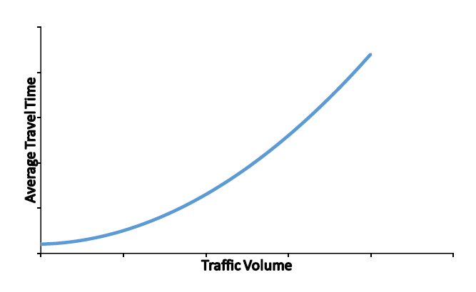
Another source of non-linearity for infrastructure management comes from flow effects. For example, roadway traffic congestion is non-linear in that a small increase in traffic may result in large amounts of delay. With roadway maintenance blocking lanes of traffic, the capacity of the roadway network is reduced and congestion may increase considerably. Figure 5.4.2 illustrates the non-linear increase in average travel time.
Non-linear optimization has some pitfalls. First, solutions obtained may not be global optimum but only local maximum or minimum values of the objective function. Second, particular formulations may lead to physically impossible results. For example, in a case of scale economies, a non-linear optimization may wish to build the top few feet of a dam rather than the entire dam since the top two feet would hold more water back than average and would be cheaper to build!
Most non-linear optimization uses some form of a gradient
approach in which a set of feasible decision variable values are
chosen and then these are altered to improve the objective function
and still remain feasible. Solver in the spreadsheet program EXCEL
uses this type of technique. In many cases, it is useful to use
multiple starting points to reduce the chance of ending up with a
local optimum.
As an example of non-linear optimization useful for infrastructure
management, we can suggest a flow problem which can be applied to
traffic flow in road networks or water flow in pipe networks. The
costs of maintenance or rehabilitation work can be estimated by
comparing flow costs before and during network disruption. The same
approach can be used for assessing new capacity or operating
procedures. The problem appears in Hendrickson (1984).
We assume that a network exists with a set of nodes (intersections) N and arcs (pipe links or streets) A. There is a cost of flow on link \(ij\) \(f(y)\) which is assumed to be monotonically increasing as in Figure 5.4.2. This assumption is physically realistic and insures convexity for the problem-solution space making a solution easier.
The general problem of equilibrium flow is:
\[P1: \text { minimize } \sum_{(i, j) \in A} \int_{0}^{x_{i j}} f_{i j}(y) d y\]
subject to:
\[\sum_{(i, k) \in A} x_{i k}-\sum_{(k, j) \in A} x_{k j}=q_{k} \text { for all } k \in N\]
\[x_{i, j}>0 \text { for all }(i, j) \in A\]
Where \(x_{ij}\) is flow on link \(ij\) and \(qk\) is the net inflow or outflow at node k. The objective is to minimize ‘impedance’ of flow on each link, and the constraints conserve flow through nodes and require all flows to be positive.
For pipeline hydraulics applications, the flow would be fluid flow measured in volume per unit time. The impedance function would be head loss (or gain) per unit of distance. The impedance function should include elevation differences of nodes as well as pipe friction loss (through a function such as the Hazen-Williams function \(f(x) = k*x^m\).
For traffic networks, a slightly more complicated form of the problem must be used to keep track of flows between particular origins and destinations. The impedance is travel time and relates to total flow on link \(ij\). Problem P2 below shows the traffic flow problem with the rs notation for traffic from node r to node s, a constraint to insure conservation of flow through intersection nodes, and a constraint to aggregate the individual origin-destination flows for each link.
\[\text {P2: minimize } \sum_{(i, j) \in A} \int_{0}^{x_{i j}} f_{i j}(y) d y\]
\[\sum_{s \in A}\left[\sum_{(i, k) \in A} x_{i k}^{r s}-\sum_{(k, j) \in A} x_{k j}^{r s}\right]=q_{r k} \text { for all } k \in N, r \in N\]
\[\sum_{s \in N}^{r \in N} x_{i j}^{r s}=x_{i j} \text { for all }(i, j) \in A\]
For the traffic flow application, the solution set of flows represents a ‘user equilibrium solution’ in which the travel time on each path used between origin r and destination s has the same overall travel time (if not, travelers would change the path and reduce their travel time). Paths not used between origin r and destination s would have higher travel time and would be unattractive.
As noted earlier, the problem P2 could be solved to obtain travel times and flows on an existing network. After the network is altered due to construction, the equilibrium travel time after the alteration could then be modelled. Noted that in this simple application form, the origin-destination flow would not change. More elaborate analysis could relax this assumption to allow new destinations or other travel choices.
Gradient solution algorithms exist for problem P1 and P2 that can easily accommodate thousands of nodes and links. Author, (Hendrickson, 1984) presents one solution algorithm as well as additional applications of the model form to project task scheduling and structural analysis. Numerous software programs exist for this type of model formulation.