4.6: Failure Rates and Survival Probabilities

In addition to deterioration models linked to component condition indexes, deterioration models may also be expressed as probabilities of failure (or survival as the inverse of failure) at different points of time. Of course, difficulty in using this approach for infrastructure components is to define what constitutes ‘failure.’ For a mechanical device such as an elevator, failure might be simply regarded as ceasing to work. For a roadway pavement, the pavement might be considered to have failed when a desired level of service is not provided, even though the roadway may still be passable at low speed.

Failure rates are defined as the likelihood of failure in the next time interval assuming that the component has not failed up until the present time. The failure rate typically is larger than the failure density function since the component has survived for one or more periods. Since infrastructure managers are concerned with forecasting the possibility of failure in the next period or two for decision making, the failure rate is generally of more interest rather than the direct probability of failure of a component at any given time in the future. We will use a numerical example to illustrate failure rates, survival probability and failure probabilities using the data shown in Table 4.6.1.

Table 4.6.1: Numerical Illustration of Failure and Survival Probabilities and Failure Rates

Period (Year)	Probability of Failure in Period \(f(t)\)	Cumulative Probability of Failure \(F(t)\)	Cumulative Probability of Survival \(R(t)\)	Failure Rate in Period \(\lambda(t)\)
1	0.10	0.10	0.90	0.100
2	0.02	0.12	0.88	0.022
3	0.02	0.14	0.86	0.023
4	0.02	0.16	0.84	0.023
5	0.02	0.18	0.82	0.024
6	0.02	0.20	0.80	0.024
7	0.10	0.30	0.70	0.125
8	0.20	0.50	0.50	0.286
9	0.20	0.70	0.30	0.400
10	0.30	1.0	0.00	1.000

Cumulative Probability of Failure \(F(t)\) is \(F(t-1) + f(t)\). Cumulative Probability of Survival R is \(1 - F(t)\). Failure rate \(\lambda(t)\) is \(\frac{f(t)}{R(t)}\) or \(R(t) - \frac{R(t-1)}{R(t)}\) .

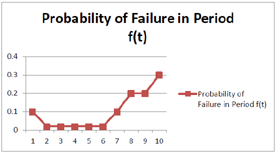
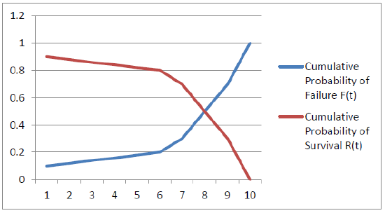
Table 4.6.1 illustrates a component that is in good condition at the present but is expected to certainly fail after ten years of use. The probability of failure f(t) (Column 2) represents an estimate of failure in each period, with a 10% of failure immediately (during a break-in period), a period of low probability of failure in years 2-6 (regular use) and then an increasing probability of failure in years 8 to 10 (wearing out). The cumulative probability of failure \(F(t)\) is the sum of failure probabilities for period \(t\) and previous periods. It begins at zero and increases steadily to 1.0 (certain failure) by year 10. Cumulative probability of survival \(R(t)\) is the inverse of the cumulative probability of failure, \(1 – F(t)\). The failure rate \(\lambda(t)\)can be calculated as:

\[\lambda(t)=\frac{f(t)}{R(t)}=R(t)-\frac{R(t-1)}{R(t)}\]

It has a value of 0.1 in period 1, reflecting the possibility of failure during the break-in period. After this, the failure rate is relatively low but increasing slowly. During the final wear our period, the failure rate increases substantially. Note that the sum of the failure rates during all periods is in excess of 1, so the failure rate is not a probability. However, for decision making, an infrastructure manager would find it helpful to know in year 5 that the risk of failure in the next period is small (0.024). However, in year 8, while the component still may be working, the risk of failure in the next period is substantial (0.400). The pattern of the failure probabilities and rates in Table 4.4.1 is common for infrastructure components and often called a ‘bathtub shape’ as illustrated in Figure 4.6.1 below.

Figure \(\PageIndex{1}\): Illustration of a Bathtub Curve. Source: By Bathtub_curve.jpg: Wyatts derivative work: McSush (Bathtub_curve.jpg) [Public domain], via Wikimedia Commons. https://commons.wikimedia.org/wiki/F...htub_curve.svg.

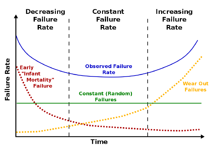
Initial break in use of a component often reveals design or fabrication flaws that may cause failure. After this break-in period, a (hopefully lengthy) period of regular use and low failure risk occurs. As the component wears out, the risk of failure increases. Figures 4.6.2 and 4.6.3 further illustrate these periods graphically for failure probability and cumulative probabilities.

Figure \(\PageIndex{2}\): Probability of Component Failure in Year t from Table 4.4.1 Data

Figure \(\PageIndex{3}\): Cumulative Probabilities of Failure and Survival from Table 4.4.1 Data

The numerical example presented above did not assume any particular distributional form for the failure probabilities. However, many applications of failure models assume some particular distribution and use historical data to estimate the parameters of the distribution. We will discuss two distributions used in this fashion: the exponential and Weibull distributions.

The form of the exponential failure model for the the cumulative probability of failure is:

\[F(t)=\int_{0}^{t} \alpha * e^{-\alpha t} d t=1-e^{-\alpha t}\]

Which is the integral from 0 to time \(t\) of the parameter α times exponential of \(-\alpha * t\) or, more simply, one minus the exponential of \(-\alpha * t\). The probability density function of failure for the exponential distributions is \(\alpha * e^{-\alpha t}\) . The exponential function has only one parameter (\(\alpha\) in this notation) and the average time to failure is the reciprocal of this parameter (\(\frac{1}{\alpha}\)). The failure rate is constant over time with a value of the parameter α (calculated from Eq. 4.6.2 as \(\alpha*\frac{e^{-\alpha t} }{e^{-\alpha t}} = \alpha \). With the negative sign in the cumulative and density failure distributions, the exponential function is often referred to as a ‘negative exponential distribution.’

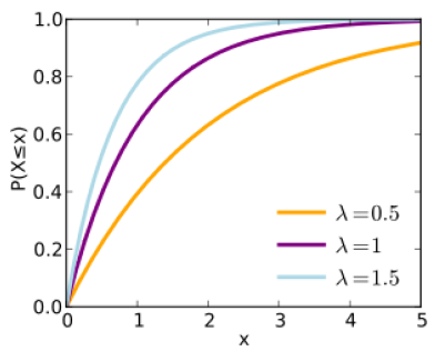
Figures 4.6.4 and 4.6.5 illustrate the form of the exponential function for different parameter values. The cumulative failure probability increases relatively rapidly initially (except for low values of the parameter \(\alpha\) continues to slowly increase for a long period of time.

Figure \(\PageIndex{4}\): Cumulative Failure Probabilities for Exponential Failure Models. Source: By Skbkekas - Own work, CC BY 3.0, https://commons.wikimedia.org/w/inde...?curid=9508326 via Wikipedia Commons, https://en.Wikipedia.org/wiki/Expone...l_distribution). This graphic uses \(\lambda\) for the distribution parameter rather than \(\alpha\), \(x\) for the time period rather than \(t\) and \(P(X \leq x)\) for \(F(t)\).

Figure \(\PageIndex{5}\): Density Probabilities for Exponential Failure Models. Source: By Skbkekas - Own work, CC BY 3.0, https://commons.wikimedia.org/w/inde...?curid=9508311 via Wikipedia Commons. This graphic uses \(\lambda\) for the distribution parameter rather than \(\alpha\), \(x\) for the time period rather than \(t\) and \(P(x)\) for \(F(t)\).

Estimation of the parameter \(\alpha\) is relatively simple in practice. Given a set of component failure observations, the parameter α is the inverse of the average time until failure observed in the sample.

A second distribution often assumed for failure models is the Weibull or ‘extreme events’ distribution. The term ‘extreme events’ reflects the use of the Weibull distribution for modelling events such as the probability of earthquakes or hurricane wind speeds. It also reflects the notion that the distribution returns the probability of the most extreme value obtained from a series of random variable results. For infrastructure components involving a large number of pieces that might fail, this analogy is appropriate. The distribution is named for Wallodi Weibull, a Swedish engineer, and mathematician who lived in the twentieth century.
The general form of the Weibull distribution includes three parameters. Using the notation of NIST (2016), the parameters are \(\mu\) (called the location parameter), \(\gamma\) (called the shape parameter) and \(\alpha\) (called the scale parameter). The failure probability density function is shown below, with \(x\) representing time:

\[f(x)=\frac{\lambda}{\alpha}\left(\frac{x-\mu}{\alpha}\right)^{(\lambda-1)} e^{\left(-\left(\frac{x-\mu}{\alpha}\right)^{\lambda}\right)} \text { where } x \geq \mu ; \lambda, \alpha>0\]

Simpler forms of the Weibull distribution function may be obtained by assuming values of the location parameter (such as \(\mu = 0\)) and the scale parameter (such as \(alpha = 1\)). Thus, one, two or three parameter forms can be obtained.

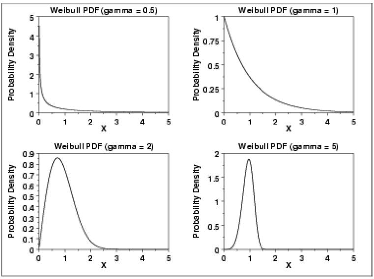
With different values of the three parameters, a wide variety of distributional forms may be obtained. Figure 4.6.6 illustrates the effects of different values of just the shape parameter.

Figure \(\PageIndex{6}\): Failure Probability Density Functions for the Weibull Distribution. Source: NIST 2016, Public Domain. Probability Density Functions for the Weibull Distribution with different values of the shape parameter (\(\gamma\) or gamma in the figure) and the location factor (\(\mu\)) zero and the scale factor (\(\alpha\)) one.