4.3: Regression Models

A more complicated approach to deterioration modelling than those in the previous section employs statistical approaches, most commonly regression analysis. These models are based upon observations of past history and conditions. The models can indicate the correlation between conditions and explanatory factors such as time and usage.

Statistical modelling is a topic of considerable interest and for which a large body of knowledge exists. In this section, we provide only the basic information that is useful for an infrastructure manager, not a researcher or expert modeler. Other works can be consulted, such as the variety of books recommended by the University of California, Berkeley, Statistics Department:

sgsa.berkeley.edu/current-stu...ommended-books

There are also a variety of software programs that can be used for statistical modelling, including add-ins to spreadsheets such as Microsoft Excel, general modelling environments such as MATLAB, or programs focused on statistical modelling such as R, S, Minitab or Statistical Package for the Social Sciences (SPSS). Any of these software programs can be used for infrastructure deterioration modelling since the data usually available for deterioration modelling are well within the capabilities of any of these software programs. Also, these programs typically provide help files and tutorials that can be consulted.

For deterioration models, the dependent variable is typically condition expressed as a numerical index. Explanatory variables may be time (such as age in years since last rehabilitation), usage, weather zone and others. Different deterioration models may be estimated for different component designs, such as pavement characteristics, or these characteristics may be added. For example, a simple linear condition model might be:

\[c=\alpha+\beta *(a g e)+\epsilon\]

where c is a condition index (such as a scale of 1 to 10), \(\alpha\) and \(\beta\) are coefficients to be estimated and \(\epsilon\) is a model error term. A series of observations of c and age would be assembled as input data for estimation. Then, a software routine could be employed to estimate the appropriate values of the coefficients \(\alpha\) and \(\beta\) for the estimated model. In these routines, the coefficients \(\alpha\) and \(\beta\) are calculated to minimize the sum of squared deviations between condition and the model forecast (represented by the \(\epsilon\) values).

Equation 4.3.1 shows a linear deterioration model, meaning that the explanatory variable age is linearly related to the dependent variable condition index. Additional explanatory variables could be added to the model, each with a coefficient to be estimated. Also, non-linear model forms can be used, such as a quadratic model where age enters as both a linear and a squared explanatory variable:

\[c=\alpha+\beta_{1} *(a g e)+\beta_{2} *(a g e)^{2}+\epsilon\]

Another common model form is an exponential model form:

\[c=\alpha *(a g e)^{\beta}\]

This exponential model is often linearized for estimation purposes by taking the logarithm of both sides of the equation to form a linear model with respect to the coefficients to be estimated:

\[\ln (c)=\alpha^{\prime}+\beta *(a g e)+\epsilon\]

Where \(\alpha '\) is the logarithm (in function) of α in Equation 4.3.2. In this linear form, the input data for estimation would be \(ln(c)\) and age.

Which model form should be chosen for use in any particular case? Generally speaking, simple forms are preferable to more complicated forms. Also, model forms that correspond to reasonable deterioration causes are preferable. For example, desirable pavement deterioration model forms would include both deteriorations over time and for different levels of vehicle usage.

As an example, Morous (2011) estimated a polynomial model of bridge deck deterioration in Nebraska based simply on bridge deck age. The estimated model was:

y=10-0.25 * x+0.0093 * x^{2}-0.0001 * x^{3}

\[y=10-0.25 * x+0.0093 * x^{2}-0.0001 * x^{3}\]

where y is condition rating (c in Eq. 4.1-4.4) and x is age (or age in Eq. 4.2.1, 4.3.1-4.3.3). As can be seen in Fig. 4.3.1, the polynomial model is close to the historical data on bridge deterioration. Morous (2011) also reports the R2 value of the estimated regression equation (equal to .99 in Figure 4.4) which is a measure of ‘goodness of fit’ of the model to the data. In this case, 99% of the variation in the dependent variable is captured by the regression model.

Figure \(\PageIndex{1}\): Deterioration History and Model of Original Bridge Decks in Nebraska. Source: Morous, 2011, UNL Digital Commons. http://digitalcommons.unl.edu/. In the model, y is condition-rating index and x is age in years.

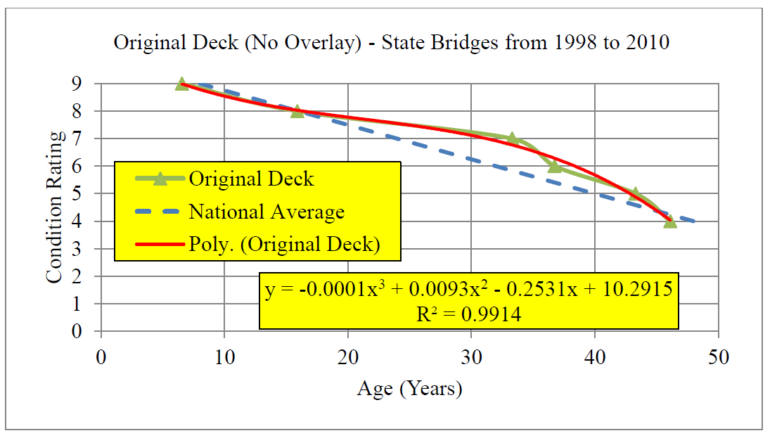
The usefulness of regression deterioration models really derives from situations in which multiple explanatory factors are of interest, such as age, pavement type and vehicle usage (generally measured in equivalent standard axle loads) for roadway pavements or bridge decks. For the model shown in Fig. 4.4, the use of historical data or the regression model has the same forecasting ability. But with more factors considered, two-dimensional graphical representations such as Fig. 4.4 cannot be used directly.

Regression approaches typically make fairly heroic assumptions about the available data and appropriate model forms. In particular, the values of the error term ε in Equations Eq. 4.2.1, 4.3.1, and 4.3.2 are generally assumed to be normally distributed with mean zero, independent of each other and with a constant variance. It is unlikely that any deterioration models fulfill these formal assumptions exactly. If nothing else, condition ratings typically are constrained to be positive, so highly negative values of ε are not allowed. Moreover, historical observations of components are unlikely to be completely independent. Fortunately, regression deterioration models are usually fairly robust, so deviation from the formal assumptions is not a practical problem to obtain reasonable coefficient estimates. However, factors such as correlated error terms make the use of formal statistical testing approaches problematic.

Forecasts from regression models are uncertain, as is the case for all deterioration models. Based on past histories and distribution assumptions, it is possible to estimate confidence intervals for forecast values. Figure 4.3.2 provides an example, with confidence intervals for Australian tax receipts shown, where a 90% confidence interval suggests that the forecast receipts will fall within the interval 90% of the time. The 90% confidence interval in this case for the following year is from 18 to 22.5 as a percent of Australian Gross Domestic Product (GDP). Developing formal confidence intervals would be unusual for infrastructure management, but the managers themselves should always be aware that the actual outcomes will likely differ from forecasts.

Figure \(\PageIndex{2}\): Forecast for Australia Tax Revenues - Example of Probability Confidence Intervals. Source: By The Commonwealth of Australia. http://www.budget.gov.au/2013-14/con...tachment_b.htm. Creative Commons BY Attribution 3.0 Australia https://creativecommons.org/licenses/by/3.0/au/. Forecast is for Australia tax revenues.