4.4: Projected Frequency and Severity and Cost-Benefit Analysis—Capital Budgeting

Learning Objectives

• In this section we focus on an example of how to compute the frequency and severity of losses (learned in "2: Risk Measurement and Metrics").
• We also forecast these measures and conduct a cost-benefit analysis for loss control.

Dana, the risk manager at Energy Fitness Centers, identified the risks of workers’ injury on the job and collected the statistics of claims and losses since 2003. Dana computed the frequency and severity using her own data in order to use the data in her risk map for one risk only. When we focus on one risk only, we work with the risk management matrix. This matrix provides alternative financial action to undertake for each frequency/severity combination (described later in this chapter). Dana’s computations of the frequency and severity appear in Table 4.1. Forecasting, on the other hand, appears in Table 4.2 and Figure \(\PageIndex{1}\). Forecasting involves projecting the frequency and severity of losses into the future based on current data and statistical assumptions.

Table 4.1 Workers’ Compensation Loss History of Energy Fitness Centers—Frequency and Severity

Year	Number of WC Claims	WC Losses	Average Loss per Claim
2003	2,300	$3,124,560	$1,359
2004	1,900	$1,950,000	$1,026
2005	2,100	$2,525,000	$1,202
2006	1,900	$2,345,623	$1,235
2007	2,200	$2,560,200	$1,164
2008	1,700	$1,907,604	$1,122
Total	12,100	$14,412,987
	Frequency for the whole period		Severity for the whole period
Mean	2,017	$2,402,165	$1,191
(See "2: Risk Measurement and Metrics" for the computation)

Table 4.2 Workers’ Compensation Frequency and Severity of Energy Fitness Centers—Actual and Trended

	WC Frequency	Linear Trend Frequency	WC Average Claim	Linear Trend Severity
2003	2,300	2,181	$1,359	$1,225
2004	1,900	2,115	$1,026	$1,226
2005	2,100	2,050	$1,202	$1,227
2006	1,900	1,984	$1,235	$1,228
2007	2,200	1,918	$1,422	$1,229
2008	1,700	1,852	$1,122	$1,230
2009	Estimated	1,786.67	Estimated	$1,231.53

Figure \(\PageIndex{1}\): Workers’ Compensation Frequency and Severity of Energy Fitness Centers—Actual and Trended

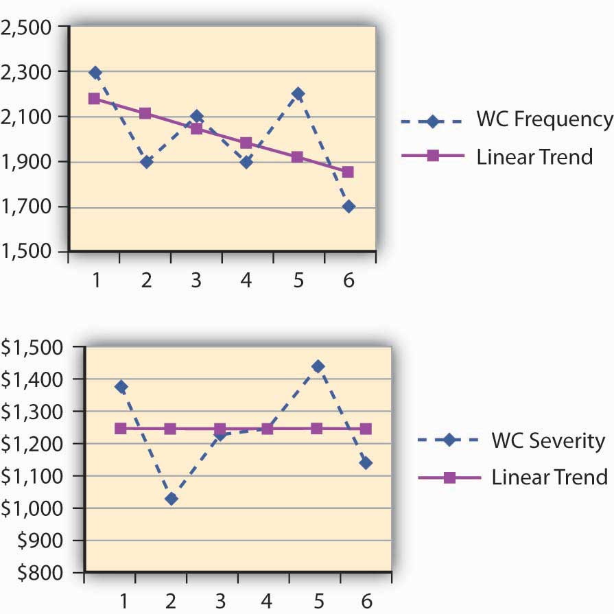
Dana installed various loss-control tools during the period under study. The result of the risk reduction investments appear to be paying off. Her analysis of the results indicated that the annual frequency trend has decreased (see the negative slope for the frequency in Figure 4.3.1). The company’s success in decreasing loss severity doesn’t appear in such dramatic terms. Nevertheless, Dana feels encouraged that her efforts helped level off the severity. The slope of the annual severity (losses per claim) trend line is 1.09 per year—and hence almost level as shown in the illustration in Figure 4.3.1. (See the "4.7: Appendix - Forecasting" to this chapter for explanation of the computation of the forecasting analysis.)

Capital Budgeting: Cost-Benefit Analysis for Loss-Control Efforts

With the ammunition of reducing the frequency of losses, Dana is planning to continue her loss-control efforts. Her next step is to convince management to invest in a new innovation in security belts for the employees. These belts have proven records of reducing the severity of WC claim in other facilities. In this example, we show her cost-benefit analysis—analysis that examines the cost of the belts and compares the expense to the expected reduction in losses or savings in premiums for insurance. If the benefit of cost reduction exceeds the expense for the belt, Dana will be able to prove her point. In terms of the actual analysis, she has to bring the future reduction in losses to today’s value of the dollar by looking at the present value of the reduction in premiums. If the present value of premium savings is greater than the cost of the belts, we will have a positive net present value (NPV) and management will have a clear incentive to approve this loss-control expense.

With the help of her broker, Dana plans to show her managers that, by lowering the frequency and severity of losses, the workers’ compensation rates for insurance can be lowered by as much as 20–25 percent. This 20–25 percent is actually a true savings or benefit for the cost-benefit analysis. Dana undertook to conduct cash flow analysis for purchasing the new innovative safety belts project. A cash flow analysis looks at the amount of cash that will be saved and brings it into today’s present value. Table 4.3 provides the decrease in premium anticipated when the belts are used as a loss-control technique.

The cash outlay required to purchase the innovative belts is $50,000 today. The savings in premiums for the next few years are expected to be $20,000 in the first year, $25,000 in the second year, and $30,000 in the third year. Dana would like to show her managers this premium savings over a three-year time horizon. Table 4.3 shows the cash flow analysis that Dana used, using a 6 percent rate of return. For 6 percent, the NPV would be \($66,310 – 50,000= $16,310\). You are invited to calculate the NPV at different interest rates. Would the NPV be greater for 10 percent? (The student will find that it is lower, since the future value of a lower amount today grows faster at 10 percent than at 6 percent.)

Table 4.3 Net Present Value (NPV) of Workers’ Compensation Premiums Savings for Energy Fitness Centers When Purchasing Innovative Safety Belts for $50,000

	Savings on Premiums	Present Value of $1 (at 6 percent)	Present Value of Premium savings
End of Year	End of Year
1	$20,000	0.943	$18,860
2	$25,000	0.890	$22,250
3	$30,000	0.840	$25,200
Total present value of all premium savings			$66,310
Net present value = \($66,310 − $50,000= $16,310> 0\)

Use a financial calculator

Risk Management Information System

Risk managers rely upon data and analysis techniques to assess and evaluate and thus to make informed decisions. One of the risk managers’ primary tasks—as you see from the activities of Dana at Energy Fitness Centers—is to develop the appropriate data systems to allow them to quantify the organization’s loss history, including

• types of losses,
• amounts,
• circumstances surrounding them,
• dates, and
• other relevant facts.

We call such computerized quantifications a risk management information system, or RMIS. An RMIS provides risk managers with the ability to slice and dice the data in any way that may help risk managers assess and evaluate the risks their companies face. The history helps to establish probability distributions and trends analysis. When risk managers use good data and analysis to make risk reduction decisions, they must always include consideration of financial concepts (such as the time value of money) as shown above.

The key to good decision making lies in the risk managers’ ability to analyze large amounts of data collected. A firm’s data warehousing (a system of housing large sets of data for strategic analysis and operations) of risk data allows decision makers to evaluate multiple dimensions of risks as well as overall risk. Reporting techniques can be virtually unlimited in perspectives. For example, risk managers can sort data by location, by region, by division, and so forth. Because risk solutions are only as good as their underlying assumptions, RMIS allows for modeling data to assist in the risk exposure measurement process. Self-administered retained coverages have experienced explosive growth across all industries. The boom has meant that systems now include customized Web-based reporting capabilities. The technological advances that go along with RMIS allows all decision makers to maximize a firm’s risk/reward tradeoff through data analysis.

KEY TAKEAWAY

• The student learned how to trend the frequency and severity measures for use in the risk map. When this data is available, the risk manager is able to conduct cost-benefit analysis comparing the benefit of adopting a loss-control measure.

Discussion Questions

1. Following is the loss data for slip-and-fall shoppers’ medical claims of the grocery store chain Derelex for the years 2004–2008.
   1. Calculate the severity and frequency of the losses.
   2. Forecast the severity and frequency for next year using the appendix to this chapter.
   3. If a new mat can help lower the severity of slips and falls by 50 percent in the third year from now, what will be the projected severity in 3 years if the mats are used?
   4. What should be the costs today for this mats to break even? Use cost-benefit analysis at 6 percent.

      Year	Number of Slip and Fall Claims	Slip-and-Fall Losses
      2004	1,100	$1,650,000
      2005	900	$4,000,000
      2006	700	$3,000,000
      2007	1,000	$12,300,000
      2008	1,400	$10,500,000