11: Homogeneous Tax Rates

Introduction

According to Benjamin Franklin, taxes are one of the two constants in life (the other one is death). Taxes need to be included in present value (PV) models because only what the firm earns and keeps after paying taxes really matters. Therefore, proper construction of PV models requires that taxes be consistently applied to defending and challenging investments.

A single-equation PV model compares two investments: a challenger, described by time-dated cash flow, and a defender, usually described by its internal rate of return (IRR) of its time-dated cash flow. Homogeneous tax rates require that the same units are used when describing the cash flow of the challenger as the cash flow used when finding the IRR of the defender. And in particular, homogeneous tax rates require that when the cash flow of the challenger are adjusted for taxes, the IRR of the defender must also be adjusted for taxes. This chapter shows how to find homogeneous tax rates in PV models.

It is popular to adjust a defender’s before-tax IRR to an after-tax IRR by multiplying it by (1 – T), where T is the average tax rate applied to the investment. This chapter points out that this method for adjusting the defender’s IRR for taxes is only appropriate in a few special cases. Finally, this chapter shows how to find appropriate tax rates for adjusting the defender’s IRR for taxes in a variety of tax environments.

After-tax PV Models for Defenders and Challengers

The goal is to find a defender’s after-tax IRR. The first step is to find the defender’s before-tax IRR. Recall that the defender’s before-tax IRR is that rate of return such that the NPV of the defender’s before-tax net cash flow is zero. The defender’s after-tax IRR discounts the defender’s after-tax cash flow so that its NPV remains equal to zero.

There is an easy test to determine if taxes have been properly introduced into a PV model. First consider the defender’s cash flow stream and its IRR. Then introduce taxes into the defender’s cash flow stream and its IRR. If taxes have been properly introduced, then the NPV of the defender’s after-tax cash flow stream discounted by its after-tax IRR is still zero.

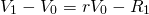
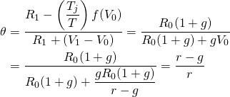
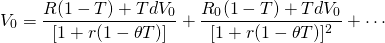
To illustrate, consider a defending investment that earns constant net cash flow of R dollars per period in perpetuity. The maximum bid (minimum sell) price V₀ for this defending investment whose before-tax IRR is r. We describe this investment in Equation \ref{11.1}.

(11.1)

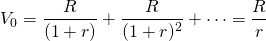
where r = R/V₀ is the before-tax IRR. Now suppose that we describe the defender’s cash flow and the IRR for this same investment on an after-tax basis. We do so by introducing the constant marginal income tax rate T into the model:

(11.2)

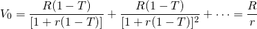
Income R and the before-tax IRR of the defender are both adjusted for taxes by multiplying by (1 – T). We can be sure that r(1 – T) is the after-tax IRR, since V₀ is the same in the before and after-tax models. However, we need to be aware that only in the special case of constant infinite income can we multiply r by (1 – T) to obtain the after-tax IRR.

A General Approach for Finding the Defender’s After-tax IRR

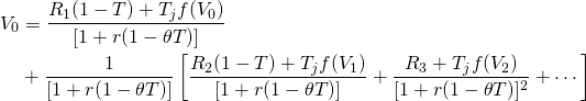
A general approach for finding the defender’s after-tax IRR follows. Consider a defender that has a market-determined value of V₀ and earns a before-tax cash flow stream of R₁, R₂, …, and whose defender’s before-tax IRR is r. A before-tax PV model for this defender can be written as:

(11.3)

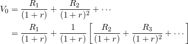
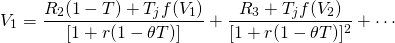
Now we express the PV model for the defender one period later as:

(11.4)

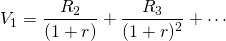
Note that the bracketed expression in Equation \ref{11.3} equals the right-hand side of Equation \ref{11.4}. This equality allows us to substitute V1 for the bracketed expression in Equation \ref{11.3}. After making the substitution in Equation \ref{11.3} we solve for capital gains equal to:

(11.5)

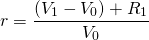
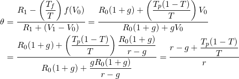
Using the expression in Equation \ref{11.5} we can solve for the defender’s before-tax IRR equal to:

(11.6)

We now want to find the after-tax IRR for the defender described in Equation \ref{11.6}. To do so, the IRR and the cash flow for the defender must be adjusted for taxes in such a way that V₀ in Equation \ref{11.3} is not changed (and the defender’s NPV is still zero). The defender’s cash flow is adjusted for taxes by multiplying them by (1 – T). The defender’s before-tax IRR is adjusted for taxes by multiplying it by where , a tax adjustment coefficient, adjusts r to its after-tax equivalent such that V₀ is the same whether calculated on a before-tax or after-tax basis. Besides these tax adjustments, let T_j equal other taxes applied to the defender’s cash flow that may include property taxes in the case of land, depreciation tax credits in the case of depreciable investments, and capital gains taxes when appropriate for assets earning capital gains. What all these taxes have in common is their functional dependence on the previous period’s asset value.

The after-tax PV model corresponding to Equation \ref{11.3} that leaves V₀ unchanged can be written as:

(11.7)

Similarly, V₁ can be expressed as:

(11.8)

Replacing the bracketed expression in Equation \ref{11.7} with V₁, we find the after-tax IRR for the defender as:

(11.9)

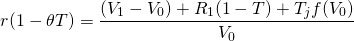
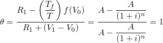
Finally, substituting for r in Equation \ref{11.9} from the right-hand side of Equation \ref{11.6} and solving for , we obtain:

(11.10)

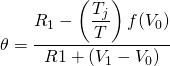
The value for in Equation \ref{11.10} adjusts the defender’s before-tax IRR to obtain homogeneity of measures between the defender’s after-tax IRR and the defender’s after-tax cash flow in Equation \ref{11.7}. When homogeneity of measures is maintained, the defender’s NPV is still zero whether calculated on a before-tax or after-tax basis. We now find some specific after-tax IRRs for various types of defenders.

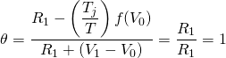
Case 11.1.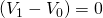 and . In this case, the defender earns neither capital gains nor suffers capital losses, in which case T_j = 0 . This case is illustrated by an infinite constant cash flow series, described in equations 11.1 and 11.2. Because the cash flow is constant, capital gains are zero. Furthermore, the defender’s return in each period is equal to its cash receipts, which is fully taxed at income tax rate T. Therefore, the entire before-tax rate of return must be adjusted by (1 – T). In Equation \ref{11.10}, substituting zero for capital gains and depreciation or capital gains tax results in:

(11.11)

Case 11.2. 0" title="Rendered by QuickLaTeX.com" height="18" width="103" style="vertical-align: -4px;"> and . In this case the investment earns capital gains that are not taxed, which lowers the defender’s effective tax rate. Thus, and . The greater the capital gains, the lower the effective tax rate in period t. We illustrate this type of model next.

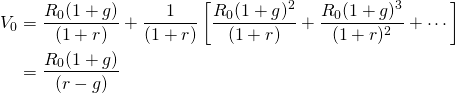
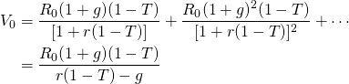
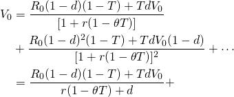
Consider a defending investment whose before-tax cash flow grows geometrically at rate g. Then before-tax cash flow in period t, R_t, equals: R₀ (1 + g)^t, and we write the investment’s IRR model as:

(11.12)

One period later, we can write:

(11.13)

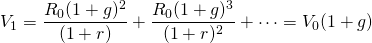
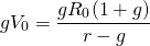
and capital gains equal:

(11.14)

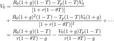
Then, substituting the right-hand side of Equation \ref{11.12} for V₀ in Equation \ref{11.14}, we obtain:

(11.15)

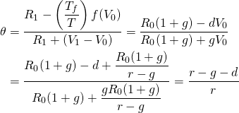
Now we are ready to find the tax-adjustment coefficient in this model. Substituting into Equation \ref{11.10} for capital gains and first period cash flow, we obtain:

(11.16)

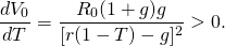
Suppose that we naively introduced taxes into the growth model described in Equation \ref{11.12} and obtained:

(11.17)

In this case, an increase in T increases V₀:

(11.18) 0. \end{equation*} " title="Rendered by QuickLaTeX.com">

Since increasing T increases V₀, we know that r(1 – T) cannot equal the after-tax IRR for the defending investment.

So what have we learned? We learned how to interpret in the geometric growth model. Earlier we demonstrated that in the geometric growth model, capital gains are earned at rate g. But in this model, capital gains are not converted to cash, and so they are not taxed. Therefore, not all earnings on the investment are taxed, only the portion earned as cash. 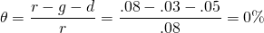As a result, the effective tax rate is not T but , where is the percentage of returns earned as cash.

If, for example, r = 8%, g = 3%, then

(11.19)

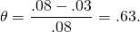
Furthermore, for an investor in the 35% tax bracket whose cash flow is increasing at 3%, the effective tax rate would be .

Case 11.3. and . In this case the investment suffers capital losses for which no tax savings are allowed, which increases the defender’s effective tax rate. Thus, 1" title="Rendered by QuickLaTeX.com" height="13" width="40" style="vertical-align: -1px;"> and 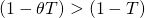(1 - T)" title="Rendered by QuickLaTeX.com" height="18" width="145" style="vertical-align: -4px;">. The greater the capital losses, the higher is the effective tax rate in period t. We illustrate this type of model next.

Consider a defending investment whose before-tax cash flow declines geometrically at rate d > 0. Then before-tax cash flow in period t, R_t, equals: , and we write the investment’s maximum bid price as:

(11.20)

One period later, we can write:

(11.21)

and capital losses equal:

(11.22)

Then, substituting the right-hand side of Equation \ref{11.20} for V₀ in Equation \ref{11.22} we obtain:

(11.23)

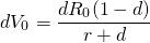
Now we are ready to find the tax-adjustment coefficient in this model. Substituting into Equation \ref{11.10} for capital losses and first period cash flow, we obtain:

(11.24)

So what have we learned? We learned that in the geometric decay model, capital losses are suffered at rate d. But since capital losses are not converted to cash, they do not create a tax shield. As a result, the effective tax rate is not T but , where is (r + d)/r which is greater than one and depends on the decay rate d. It should be obvious that the two previous cases are equivalent since d could be replaced by g < 0. On the other hand, it may be helpful later on to distinguish between growth in cash receipts g% and book value depreciation d%.

If for example, r = 8%, d = 3%, then,

(11.25)

Furthermore, for an investor in the 35% tax bracket, the effective tax rate on cash flow described by a geometric growth pattern would be 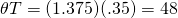The conclusion of Case 11.3 is that suffering losses on investments which are not used to shield income from taxes increases the investor’s effective tax rate.

Case 11.4.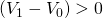 0 " title="Rendered by QuickLaTeX.com" height="18" width="103" style="vertical-align: -4px;"> and 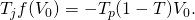In this model, the defending investment earns capital gains but pays property tax on its previous period’s value times the property tax rate T_p. However, property taxes are tax deductible, so we can write the after-tax IRR model for the defending land investment as:

(11.26)

We can sum the IRR model above by recognizing that it consists of two geometric sums. However, after summing, V₀ appears on both sides of the equation. Therefore, we solve for V₀ using Equation \ref{11.26} and obtain:

(11.27)

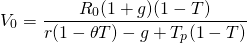
Capital gains and V₀ in this model are the same as in Case 11.2, which allows us to write:

(11.28)

Consider the effect of property taxes compared to the geometric model without property taxes. In Case 11.2, we assumed that r = 8% and g = 3%, so that . We continue with the assumption that the decision maker is in the 35% tax bracket and add the assumption that the property tax rate is 2%. We now substitute into Equation \ref{11.28} and find:

(11.29)

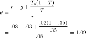
So what have we learned? We learned that property taxes increase the effective tax rate. To illustrate, for an investor in the 35% tax bracket, the effective tax rate on cash flow described by a geometric growth pattern with property taxes would be . Obviously, property taxes increase an investor’s effective tax rate.

Case 11.5. 0" title="Rendered by QuickLaTeX.com" height="18" width="103" style="vertical-align: -4px;"> and 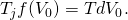A most fortuitous tax environment is an investment that appreciates but is considered to depreciate at rate d for tax purposes. In this case the investor is not required to pay taxes on the capital gains and is allowed a tax credit for depreciation that occurs only on the books. An example of such a model is the following:

(11.30)

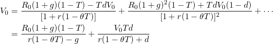
Because the before-tax model is the geometric growth model, we can write:

(11.31)

To illustrate, suppose that d = 5%. Then, using numbers from our previous example, we substitute into Equation \ref{11.31} and find:

(11.32)

In other words, the tax rate for the investment is effectively zero.

Tax Adjustment Coefficients in Finite Models

So far we have obtained tax adjustment coefficient models for infinite time examples. As a result, the tax adjustment coefficients have been the same for each period. This approach has been convenient for exposition purposes. However, this result is not generally applicable. In practice, the tax adjustment coefficients vary by time period. We demonstrate using a finite time horizon model, a loan model in which the interest paid is tax deductible.

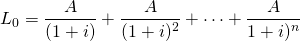
In many applications, the defender is a loan. When a loan is the defender, we immediately want to know if the interest paid is tax deductible. To keep our analysis simple, assume a constant-payment loan made for n periods at an interest rate of i percent. In which case, loan amount L₀ at interest rate i with annuity payments A can be written as:

(11.33)

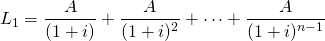
And the firm’s before-tax IRR is i. The loan balance after one period can be written as:

(11.34)

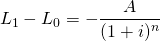
Furthermore, capital loss for loans can be expressed as:

(11.35)

The after-tax IRR model can be expressed as:

(11.36)

With Equation \ref{11.36} in a familiar form, we can write as:

(11.37)

In words, the effective after-tax IRR for a loan whose interest is tax-deductible is (1 – T).

Ranking Investments and Taxes

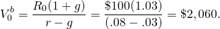
In this section, we acknowledge that the effective tax rates vary by the different types of investments being considered. Furthermore, if the effective tax rate for defenders and challengers differ, then before and after-tax investment rankings may be changed. To make this point, consider the following example. Assume the defender’s before-tax IRR is 8%, the income tax rate is 35%, the rate of growth in net cash flow is 3%, and the last year’s before-tax net cash flow was $100. The maximum bid price for this investment with geometric growing income is:

(11.38)

If the minimum sell price is $3,000, then the NPV for the investment is a negative $940 and the challenger is rejected.

Now suppose we introduce taxes into the model and recalculate the investment’s NPV. To simplify we assume an infinite life for the investment and assume for the defender and find:

(11.39)

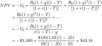
Now the challenger’s NPV is positive. Introducing taxes into the NPV model has reversed the ranking: the challenger is now preferred to the defender. These results should alert financial managers to the importance of after-tax rankings.

Summary and Conclusions

Taxes are important when valuing and ranking investments because what really matters is the amount of your earnings you get to keep after paying taxes. It’s not the before-tax IRR that matters but the after-tax IRR that counts because that’s the rate you really earned on your defending investment.

In this chapter, we have introduced a method for finding a defender’s after-tax IRR. The method required that when a defender’s cash flow adjusted for taxes and was discounted by its after-tax IRR its change in NPV was zero. Then we used the equality to find the after-tax discount rate IRR. The implied tax rate in the after-tax IRR was compared to the firm’s average marginal income tax-rate.

While the usual practice is to multiply the defender’s before-tax IRR by (1 – T) to obtain the defender’s after-tax IRR, this chapter demonstrated that this cannot be generally relied on to obtain the defender’s properly adjusted after-tax IRR. Indeed, we demonstrated that capital gains that are not taxed can lower the effective tax rate. Capital losses that do not create tax shields can increase the effective tax rate. Property tax paid on land and other real property increases the effective tax rate paid. Allowing investors to write off an investment’s depreciation lowers the effective tax rate.

Finally, this chapter has employed simplifying assumptions, such as large values for n and average depreciation and growth rates, to find effective after-tax discount rates that have nice, closed-form solutions. Usually, this is not the case. It is often more difficult to find effective after-tax discount rates, and often these are not closed-form solutions.

Questions

1. Describe the appropriate test for determining whether or not taxes have been properly introduced into the defender’s IRR.
2. When finding after-tax IRRs for defenders, we solve for and claim that is the defender’s effective tax rate. Interpret the meaning of .
3. Under what condition is the defender’s effective tax rate equal to its income tax rate T or that ?
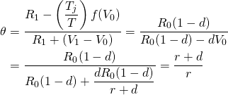
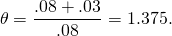
4. Assume that a defending investment’s price is V₀, that d is the defender’s book value depreciation rate, that R is the constant stream of income earned by the defender, that T is the income tax rate, and that r is the defender’s before-tax IRR. Also assume that the defender is allowed to write off book value depreciation even though its income stream is constant. We write such a model as:

(Q11.1)

In this model, the depreciation is constant for 100/d periods beyond which the discounted cash flow is small enough to be ignored. The before-tax IRR model can be written as:

(Q11.2)

Solve for in the after-tax IRR model by substituting for V₀ the right hand side of the second model R/r. Next, solve for a numerical value for assuming that d = 3% and r = 8%.

5. Suppose that you have found the NPV for a challenger. What impact will an increase in the defender’s effective tax rate have on the challenger’s IRR? Please explain your answers.
6. Calculate the effective tax rate for a depreciating challenger where d is the depreciation rate, T is the income tax rate, r is the defender’s before-tax IRR, and V₀ is the price of defender. The IRR model is written below. (Hint: find by setting the right hand side of the equation below to the equivalent model without taxes (T = 0) and solve for .

(Q11.3)

7. Discuss the following. Suppose that cash flow was constant (R_t = R₀), yet tax laws allowed the owner of the durable to claim depreciation at rate d. Without solving for , can you deduce whether it would be equal to, less than, or greater than one? Defend your answer.
8. Assume you are investing in land and that you borrow money to finance its purchase. Also assume that you pay property taxes on the land. In other words, land is the challenger and the loan is the defender. Which investment has the higher effective tax rate under three scenarios: g = 0, g > 0, and g < 0? What do you need to know about the property tax rate T_p to answer this question?
9. In this chapter, five different investment tax scenarios were described. Please provide an example of each type of investment and how the tax scenario might change its rankings compared to before-tax rankings.