
6: System Analysis
- Page ID
- 12751

After completing this chapter, you should be able to (1) define a system; (2) recognize system properties included in coordinated financial statements (CFS); and (3) connect changes in exogenous variables determined outside the CFS system to changes in endogenous variables calculated inside the CFS system to answer”what if” and “how much” kinds of questions.
To achieve your learning goals, you should complete the following objectives:
- Learn what is a system
- Learn how CFS satisfy system requirements.
- Learn how individual financial statements included in the CFS are connected.
- Learn how subsystems can be created from a system.
- Learn how to answer the question: what if the value of an exogenous variable included in the CFS system changes, then how will the values of endogenous variables included in the CFS change?
- Learn how to answer the question: how much does the value of an exogenous variable included in the CFS system need to change for the value of a specified endogenous variable included in the CFS to equal a specified value?
- Learn how asking what if and how much questions about changes in exogenous variables allows firm managers to conduct opportunity and threat analysis.
- Learn how to create a subsystem of the CFS system that describes a firm’s rate of return on equity (ROE).
- Learn how to create a subsystem of the CFS system that describes a firm’s solvency.
- Learn how to compute common size balance sheets and accrual income statements (AIS) and describe the trade-off perspectives they provide.
Introduction
In what follows we define a system and distinguish between the different kinds of systems. Then we make the point that CFS are a system.
CFS are a system. Indeed we have already used the system properties of CFS to answer the question: “what is” the financial condition of the firm? We answered that question by constructing ratios that described the firm’s (S)olvency, (P)rofitability, (E)fficiency, (L)iquidity, and (L)everage (SPELL) ratios. However, the value of information gained from SPELL ratios has its limit. Answering “what is” kinds of questions is a static (timeless) analysis because its focus is on the current financial condition of the firm. We need addition information that is forward looking such as knowing how the financial condition of the firm may change in response to changes in the external environment of the firm. We may also want to know what kinds of changes are required in the firm’s external environment for specified changes to occur within the CFS system.
Because CFS is a system, we can use it as our primary strengths, weaknesses, opportunities, and threats analysis tool. We summarize several reasons why the system’s properties of CFS are important for financial managers conducting strengths, weaknesses, opportunities, and threats analysis:
- Because it allows us to answer the question: what is the financial condition of the firm reflected by its SPELL ratios. Answering the what is question is the primary means for conducting strengths and weakness analysis.
- Because the relationships between CFS variables and financial statements are consistent (they don’t change and cannot produce a contradiction), we can check the accuracy of our numbers by looking for extraordinary numbers in the statements. If we observe unrealistic results, they can only be attributed to the data’s inaccuracy.
- Because it allows us to ask what if questions by changing conditions in the external environment of the firm and noting changes in the financial condition of the firm. Answering what if questions is one of two primary means for conducting opportunities and threats analysis.
- Because it allows us to ask how much questions and determine how much of an external change is needed to change a particular variable inside the system. Answering how much questions is one of two primary means for conducting opportunities and threats analysis.
- Because it allows us to define subsystems to focus on parts of the system such as profitability and solvency that we want to emphasize.
Coordinated Financial Statements as a System
What is a system. A system is an interacting and interdependent group of items forming a unified whole and serving a common purpose (Wikipedia). Every system has boundaries that separate activities that occur within the system from those that occur outside of the system. Each element of the system contributes to a common purpose.
There are, of course, several kinds of systems. An abstract system uses variables to represent tangible or intangible things and may or may not have a real world counterpart. On the other hand, physical systems are generally concrete operational systems made up of people, materials, machines, energy, and other physical things. Physical systems are the actual systems that abstract systems may attempt to represent.
Finally, systems may be closed or open. Open systems allow for exogenous forces outside of the system to influence endogenous activities within the firm. Closed systems are immune to exogenous forces. Finally, systems may be stochastic such that endogenous outcomes within the system can only be described with probabilities. Meanwhile deterministic systems are connected endogenously and exogenously with certain (non probabilistic) relationships.
Coordinated financial statements are a system. The CFS are an abstract system whose variables and statements are described using mathematical equations and numbers. The CFS are designed to represent the financial condition of the firm at the beginning and ending of a period with balance sheets and financial activities between the beginning and ending balance sheets using an accrual income statement (AIS) an a statement of cash flow (SCF). The CFS are an open system. They allow for an external environment represented by exogenous variables to influence activities within the firm represented by endogenous variables. Finally, for our purposes, we assume that the relationships between financial statements and variable values included in the CFS system are deterministic.
To understand the CFS system, we must be able to distinguish between endogenous and exogenous variables. One easy way to distinguish between CFS’ endogenous and exogenous variables is to ask: was this variable calculated somewhere in the system? Or was this variable’s value determined outside of the system? If the variable was calculated within the system, it is an endogenous variables. If the variable was calculated outside of the system, it is an exogenous variable. A firm’s coordinated financial statements for a given time period includes its end-of-period balance sheets, an (accrual) income statement (AIS), and a statement of cash flow (SCF). The firm’s CFS constitute a system because their endogenous and exogenous variables are interdependent. The variables are connected with equations that describe how the endogenous variables are calculated and how the financial statements are connected.
To illustrate, cash balances in the previous period’s ending balance sheet is an exogenous variable. It’s value was determined by activities in previous time periods. In contrast, the current period’s ending period cash balances depend on cash balances at the end of the previous period and changes in cash position calculated in the SCF. Therefore the firm’s cash balance in the current period’s ending balance sheet is an endogenous variable.
Endogenous and exogenous variables create interdependencies between the financial statements in the CFS system. In general, financial activities described in the AIS and statement of cash flow link the beginning and ending balance sheets. To illustrate:
1) Change in cash position calculated in the statement of cash flow equals the difference in cash and marketable securities recorded in the beginning and ending period balance sheets.
2) Cash flow from changes in notes and long-term liabilities in the beginning and ending period balance sheets equal cash flow recorded in the financing section of the statement of cash flow.
3) Addition to retained earning calculated in the AIS equals the difference between the firm’s retained earnings recorded in the beginning and ending period balance sheets.
Over identified variables and systems. We discussed over identified variables in Chapter 4. We review and illustrate the concept again here. Suppose that we use the system properties of the CFS to find the ending period cash balances. Then suppose we observe that the ending cash balance calculated as an endogenous variable in our balance sheet is different than the ending cash balance in our check book.
The problem is that the ending cash balance value is over identified. It can be calculated as an endogenous variable within the financial system or observed externally as an exogenous variable. When the two values differ, we say the system is inaccurate because exogenously and endogenously variable values differ from one another and the financial manager must employ his/her best effort to find the error in the data. Resolving data errors revealed by over identified variables may be the most challenging task facing financial managers whose data is often incomplete and not always accurate. Sometimes the data errors revealed by over identified variables provides financial managers the opportunity to encourage the principals of the firm to reexamine their financial records and look for errors or missing data.
Prioritizing Opportunities and Threats Questions
Financial ratios. Chapter 5 described the financial system of the firm using SPELL ratios. Of course the ratios in each of the SPELL categories provide some information by themselves. Alone, they help us answer what is the financial condition of the firm and what are its strengths and weaknesses. However, ratios are more useful when their interdependence is recognized. In other words a change in the firm’s solvency is likely to change the firm’s liquidity. A change in the firm’s efficiency is likely to change the firm’s profitability. And the list of possible interdependencies continues. Since the variables in the financial system are interdependent, the ratios composed of system variables are also interdependent.
How do we proceed to examine the interdependencies of the firm? We limit and organize our examination of the financial interdependencies by focusing on the firm’s bottom line—its profitability ratios.
A firm can exist for many reasons. It may satisfy the firm owners’ desires to engage in a particular production activity. (For example, I just want to farm!) It may be organized to provide family members and others employment. It may exist to provide some public service. There are undoubtedly other reasons why firms exist. But, the firm financial manager is charged with only one mission—to ensure the firm’s survival and its profitability. This requires a proper balance at least between the firm’s return and its solvency.
In this view, solvency ratios described by the times interest earned (TIE) and debt-to-service (DSR) ratios and profitability ratios described by margin (m), return on equity (ROE), and return on asset (ROA) ratios are the most important of the SPELL ratios. However, efficiency, leverage, and liquidity ratios also matter to the firm because they influence its profitability measured by its ROE and ROA ratios and its solvency measured by its TIE and DSR ratios. One such formula that connects the firm’s profitability ratios and other considerations of the firm including leverage and efficiency is the DuPont equation introduced in Chapter 5.
System Metaphors
A metaphor compares two ideas or objects that are dissimilar to each other in some ways and similar to each other in other ways. We use three metaphors to describe how changes in an exogenous variable—a shock—change endogenous variables.
Balloons. One might compare the CFS to a balloon. If you squeeze one part of the balloon (an exogenous force), there will be an (endogenous) bulge somewhere else in the balloon. This action-reaction nature of a system (and balloons) leads to us examine shocks in pairs and answer the question: “what if” a change in an exogenous variable occurs, “then” what happens to the endogenous variables of the system?
Predicting the weather. Predicting the financial future of the firm has characteristics in common with predicting the weather. Meteorologists look at where the weather fronts have been, the direction they have been traveling, and then predict where they will likely be in the future. To hedge their bets, they often predict future weather patterns with probabilities. Predicting the future financial condition of the firm also looks at the condition of the firm now, how it has changed over time, and then predicts with probabilities where it will be in the future.
The detective. Trying to describe how changes in an exogenous variable will affect endogenous variables is like a detective trying to put all the clues together to solve a case that explains who committed the crime. The detective observes a crime—a condition different than what existed before the crime occurred. The financial manager observes changes in the firm’s endogenous variables and attempts to link them to changes in one of the exogenous variables.
CFS systems are not unique because every financial system may define its endogenous and exogenous variables differently. As a result, each system may define its interdependencies differently, which in turn defines how consistency is achieved in the system. Nevertheless, a template that describes the system may be our best and only approach for answering system-wide what if and how much types of questions.
What If Analysis
At the beginning of this chapter, we emphasized how endogenous and exogenous variables created interdependence in the CFS system. Therefore, any change in an exogenous variable in one part of the CFS system will produce changes in endogenous variables in other parts of the system. Tracing the impact of a change in an exogenous variable on endogenous variables in the system is referred to here as what if analysis. The exogenous variable changed by the analyst is often referred to as a control variable—a special kind of exogenous variable.
What if analysis can be helpful in several ways. First, changes in exogenous variables outside of the firm’s control may be examined by following their consequences throughout the CFS system. This exercise helps the firm anticipate and plan for different outcomes. A second benefit that may be derived from what if analysis is that changes in exogenous variables may reflect the need for alternative financial strategies that can be evaluated before being adopted and those most beneficial to the firm can be adopted.
The first step in the what if analysis is to introduce the change in an exogenous or control variable. The second step is to recalculate the endogenous variables in the financial statements. The third step is to recalculate the SPELL ratios and compare them to the previous ratio values and to industry averages. And finally, the fourth step is to interpret the results which should include describing connections between changes in the firm’s SPELL ratios. Fortunately, steps one, two, and three can be automated using Excel spreadsheets.
To help analyze the changes in exogenous variables described in the scenarios below, we use an Excel integrated set of financial statements described in this chapter. The Excel spreadsheet describes HQN’s coordinated financial system and allows those interested in answering what if questions to substitute actual numbers and note the changes in absolute values in the financial statements and ratios.
To illustrate what if analysis, consider the following change in an exogenous variable. Suppose cash receipts for HQN were $39,990 instead of $38,990. The changes that result in HQN’s financial statements are highlighted in Table 6.1. As a result of an increase in cash receipts reported in the statement of cash flow (an exogenous variable), EBIT and EBT increased by $1,000. Taxes increased by 40% of the increased earning, from $58 to $468. NIAT increased by $600 of after-tax income to $702 as did retained earnings. Finally assets and equity and liabilities all increased by $600 of after-tax income.
Table 6.1. Coordinated
Financial Statements for Hi-Quality Nursery Cash Receipts =
$39,990
Open Table 6.1 in Microsoft
Excel
| BALANCE SHEET | ACCRUAL INCOME STATEMENT | STATEMENT OF CASH FLOW | ||||||
| DATE | 12/31/2017 | 12/31/2018 | DATE | 2018 | DATE | 2018 | ||
| Cash and Marketable Securities | $930 | $1,200 | + | Cash Receipts | $39,990 | + | Cash Receipts | $39,990 |
| Accounts Receivable | $1,640 | $1,200 | + | Change in Accounts Receivable | ($440) | – | Cash Cost of Goods Sold | $27,000 |
| Inventory | $3,750 | $5,200 | + | Change in Inventories | $1,450 | – | Cash Overhead Expenses | $11,078 |
| Notes Receivable | $0 | $0 | + | Realized Cap. Gains/Depr. Recapture | $0 | – | Interest paid | $480 |
| Total Current Assets | $6,320 | $7,600 | Total Revenue | $41,000 | – | Taxes | $468 | |
| Depreciable Assets | $2,990 | $2,710 | + | Cash Cost of Goods Sold | $27,000 | Net Cash Flow from Operations | $964 | |
| Non-depreciable Assets | $690 | $690 | + | Change in Accounts. Payable | $1,000 | + | Realized Cap. Gains + Depr. Recapture | $0 |
| Total Long-Term Assets | $3,680 | $3,400 | + | Cash Overhead Expenses | $11,078 | + | Sales Non-depreciable Assets | $0 |
| TOTAL ASSETS | $10,000 | $11,000 | + | Change in Accrued Liabilities | ($78) | – | Purchases Non-depreciable Assets | |
| Notes Payable | $1,500 | $1,270 | + | Depreciation | $350 | + | Sale Depreciable Assets | $30 |
| Current Portion Long-Term Debt | $500 | $450 | Total Expenses | $39,350 | – | Purchases Depreciable Assets | $100 | |
| Accounts Payable | $3,000 | $4,000 | Earnings Before Interest and Taxes (EBIT) | $1,650 | Net Cash Flow from Investment | ($70) | ||
| Accrued Liabilities | $958 | $880 | – | Less Interest Costs | $480 | + | Change in Non-Current Long Term Debt | ($57) |
| Total Current Liabilities | $5,958 | $6,600 | Earnings Before Taxes (EBT) | $1,170 | + | Change in Current Portion of Long Term Debt | ($50) | |
| Non-Current Long-Term Debt | $2,042 | $1,985 | – | Less Taxes | $468 | + | Change in Notes Payable | ($230) |
| TOTAL LIABILITIES | $8,000 | $8,585 | Net Income After Taxes (NIAT) | $702 | – | Less Dividends and Owner Draw | $287 | |
| Contributed Capital | $1,900 | $1,900 | – | Less Dividends and Owner Draw | $287 | Net Cash Flow from Financing | ($624) | |
| Retained Earnings | $100 | $515 | Addition to Retained Earnings | $415 | CHANGE IN CASH POSITION | $270 | ||
| Total Equity | $2,000 | $2,415 | ||||||
| TOTAL LIABILITIES AND EQUITY | $10,000 | $11,000 | ||||||
Table 6.2. HQN Ratio
Analysis after a $1,000 increase in Cash Receipts
Open Table 6.2 in Microsoft Excel
| Ratios | Industry Average | Activity Ratios | HQN Base | Increase CR by $1000 |
| Solvency | ||||
| TIE | 2.50 | 3.44 | 1.35 | 3.44 |
| DSR | 1.40 | 2.04 | 1.02 | 2.04 |
| Profitability | ||||
| ROA | 3.30% | 16.50% | 6.50% | 16.50% |
| ROE | 10.70% | 58.50% | 8.50% | 58.50% |
| m margin | 29.00% | 2.85% | 0.43% | 2.85% |
| Efficiency | ||||
| ITO | 7.7 | 10.93 | 10.67 | 10.93 |
| ITOT | 47.4 | 33.38 | 34.22 | 33.38 |
| ATO | 3.2 | 4.10 | 4.00 | 4.10 |
| ATOT | 114.1 | 89.02 | 91.25 | 89.02 |
| RTO | 11.41 | 25.00 | 24.39 | 25.00 |
| RTOT | 32 | 14.60 | 14.97 | 14.60 |
| PTO | 12.59 | 9.33 | 9.33 | 9.33 |
| PTOT | 29 | 39.11 | 39.12 | 39.11 |
| Liquidity | ||||
| Current Ratio | 1.30 | 1.06 | 1.06 | 1.06 |
| Quick Ratio | 0.70 | 0.43 | 0.43 | .43 |
| Leverage | ||||
| Debt/Assets | 0.91 | 0.80 | 0.80 | .8 |
| Debt/Equity | 2.00 | 4.00 | 4.00 | 4.00 |
| Asset/Equity | 2.20 | 5.00 | 5.00 | 5.00 |
In Chapter 5, we focused on ratio analysis. As a result of changes from increased cash receipts, we ask: how many ratios calculated in the previous chapter change? In other words, compare the new and old ratios. The new ratios resulting from an increase in CR of $1,000 are reported in the activity column in Table 6.2. Compare these to the HQN base ratios. The TIE solvency ratio increased from 1.35 to 3.44. The ROA profitability ratio increased from 6.5% to 16.5%. The ITO efficiency ratio increased from 10.67 to 10.93. Liquidity and leverage ratios that depend on beginning balance sheet values remain unchanged. Based on the changes in SPELL ratios resulting from an increase of $1,000 in CR, life is good at HQN!
What If Analysis and Scenarios
In what follows, we describe several scenarios facing HQN that could be analyzed by changing exogenous variables and noting their effect on CFS endogenous variables. Obviously, each of the changes has the capacity to produce changes in HQN’s SPELL ratios. Following these consequences throughout the financial system, a what if analysis exercise, is really answering the question: what if something happens, then what?
What complicates our scenario analysis is that more than one exogenous variable change may be required to answer the what if question. Consider several scenarios that we describe next.
Scenario 1. The firm has not been replacing its long-term assets. As a result, its cost of goods sold has been increasing due to increased repairs and maintenance. What are the consequences of this scenario on the financial condition of the firm?
Scenario 2. A financial manager is risk-averse and decides to increase the firm’s current assets. What actions can the firm manager take to increase the firm’s level of current assets. What are the consequences of increasing the firm’s current assets relative to its fixed assets?
Scenario 3. Suppose the firm decides to increase the time it takes to repay its notes payable. What are the advantages/disadvantages of adopting such a strategy? What conditions facing the firm might prompt it to increase the time it takes to repay its notes payable? What ratios would you want to investigate to confirm your assumptions?
Scenario 4. To boost its cash receipts, the firm offers easy credit terms to its customers. What are the implications for the firm? How would you expect the firm’s credit policies to be reflected in the firm’s financial statements?
Scenario 5. Market conditions have reduced the demand for the firm’s products. As a result, cash receipts are falling. Unfortunately, most of the firm’s costs are fixed and don’t adjust to changing output levels. What changes would you expect to find in future financial statements of the firm?
Scenario 6. The firm’s owners face serious medical costs and must extract funds from the business. Describe the impact of these expenses on the firm’s financial statements.
Scenario 7. The firm makes a major investment in long-term assets to improve its efficiency. One impact of the change is to reduce its taxes because of the increased depreciation. Describe other consequences on the firm’s financial statements.
Scenario 8. Hard economic times have reduced the firm’s customers’ ability to pay for their purchases in the usual amount of time. Describe the consequences on the firm’s financial statements.
Scenario 9. Cash receipts have been inadequate for the firm to meet its notes payable and current long-term liabilities. As a result, it is forced to sell off some of its long-term assets at values less than reported on its balance sheet. What other strategies can the firm adopt to meet its solvency demands?
Scenario 10. Reduced cash receipts without changes in production levels have led to increased inventories. To meet its financial demands, the firm has restructured its debt, decreasing the current portion of the long-term debt. How will these changes be reflected in its financial statements?
Scenario 4 illustration. Consider performing what if analysis on scenario 4. The analysis requires that we assume specific numbers. In our illustration assume that CR increased by 5% from $38,990 to $40,940. Then, because production has increased, assume that cash COGS increase by 8% from $27,000 to $29,160. There may be other changes in exogenous variables, but these are sufficient to illustrate our scenario analysis. After making the changes, we resolve the CFS template and report the consequences in the activity column. In case we want to save our results for later analysis, we save them under scenario 4 column in Table 6.3 below.
Table 6.3. HQN’s SPELL
Analysis for Scenario 4.
Open Table 6.3 in Microsoft Excel
| Ratios | Industry Average | Activity Ratios | HQN Base | Scenario 4 |
| Solvency | ||||
| TIE | 2.50 | 0.92 | 1.35 | 0.92 |
| DSR | 1.40 | 0.81 | 1.02 | 0.81 |
| Profitability | ||||
| ROA | 3.30% | 4.40% | 6.50% | 4.40% |
| ROE | 10.70% | -2.00% | 8.50% | -2.00% |
| m margin | 29.00% | -0.10% | 0.43% | -0.10% |
| Efficiency | ||||
| ITO | 7.7 | 11.19 | 10.67 | 11.19 |
| ITOT | 47.4 | 32.63 | 34.22 | 32.63 |
| ATO | 3.2 | 4.20 | 4.00 | 4.20 |
| ATOT | 114.1 | 87.01 | 91.25 | 87.01 |
| RTO | 11.41 | 25.58 | 24.39 | 25.58 |
| RTOT | 32 | 14.27 | 14.97 | 14.27 |
| PTO | 12.59 | 10.05 | 9.33 | 10.05 |
| PTOT | 29 | 36.31 | 39.12 | 36.31 |
| Liquidity | ||||
| Current Ratio | 1.30 | 1.06 | 1.06 | 1.06 |
| Quick Ratio | 0.70 | 0.43 | 0.43 | 0.43 |
| Leverage | ||||
| Debt/Assets | 0.91 | 0.80 | 0.80 | 0.80 |
| Debt/Equity | 2.00 | 4.00 | 4.00 | 4..00 |
| Asset/Equity | 2.20 | 5.00 | 5.00 | 5.00 |
While HQN successfully increased its CR, its ROA decreased from 6.5% to 5.6% and its ROE decreased from 8.5% to 3.98%. A homework exercise asks you to examine other consequences of increases in CR and COGS. However, one lesson learned from this scenario analysis is to be careful what you wish for—especially if your ultimate goal is to increase the profitability of your firm.
How Much Questions and Goal Seek
CFS system’s properties allow us to ask and answer important what if kinds of questions by changing an exogenous variable and observing its effect on the endogenous variables of the system. Goal Seek is an important Excel function that allows us to ask and answer how much kinds of questions. How much questions take the form: how much change is required in an exogenous variable x for variable y to reach a particular value, a goal, equal to a? To illustrate using HQN data, suppose we asked: how much must HQN’s CR increase for ROE to equal 9%?
Table 6.4. Coordinated
Financial Statements for Hi-Quality Nursery
Open Table 6.4 in Microsoft Excel
| BALANCE SHEET | ACCRUAL INCOME STATEMENT | STATEMENT OF CASH FLOW | ||||||
| DATE | 12/31/2017 | 12/31/2018 | DATE | 2018 | DATE | 2018 | ||
| Cash and Marketable Securities | $930 | $606 | + | Cash Receipts | $39,000 | + | Cash Receipts | $39,000 |
| Accounts Receivable | $1,640 | $1,200 | + | Change in Accounts Receivable | ($440) | – | Cash Cost of Goods Sold | $27,000 |
| Inventory | $3,750 | $5,200 | + | Change in Inventories | $1,450 | – | Cash Overhead Expenses | $11,078 |
| Notes Receivable | $0 | $0 | + | Realized Cap. Gains/Depr. Recapture | $0 | – | Interest paid | $480 |
| Total Current Assets | $6,320 | $7,006 | Total Revenue | $40,010 | – | Taxes | $72 | |
| Depreciable Assets | $2,990 | $2,710 | + | Cash Cost of Goods Sold | $27,000 | Net Cash Flow from Operations | $370 | |
| Non-depreciable Assets | $690 | $690 | + | Change in Accounts. Payable | $1,000 | + | Realized Cap. Gains + Depr. Recapture | $0 |
| Total Long-Term Assets | $3,680 | $3,400 | + | Cash Overhead Expenses | $11,078 | + | Sales Non-depreciable Assets | $0 |
| TOTAL ASSETS | $10,000 | $10,406 | + | Change in Accrued Liabilities | ($78) | – | Purchases Non-depreciable Assets | |
| Notes Payable | $1,500 | $1,270 | + | Depreciation | $350 | + | Sale Depreciable Assets | $30 |
| Current Portion Long-Term Debt | $500 | $450 | Total Expenses | $39,350 | – | Purchases Depreciable Assets | $100 | |
| Accounts Payable | $3,000 | $4,000 | Earnings Before Interest and Taxes (EBIT) | $660 | Net Cash Flow from Investment | ($70) | ||
| Accrued Liabilities | $958 | $880 | – | Less Interest Costs | $480 | + | Change in Non-Current Long Term Debt | ($57) |
| Total Current Liabilities | $5,958 | $6,600 | Earnings Before Taxes (EBT) | $180 | + | Change in Current Portion of Long Term Debt | ($50) | |
| Non-Current Long Term Debt | $2,042 | $1,985 | – | Less Taxes | $72 | + | Change in Notes Payable | ($230) |
| TOTAL LIABILITIES | $8,000 | $8,585 | Net Income After Taxes (NIAT) | $108 | – | Less Dividends and Owner Draw | $287 | |
| Contributed Capital | $1,900 | $1,900 | – | Less Dividends and Owner Draw | $287 | Net Cash Flow from Financing | ($624) | |
| Retained Earnings | $100 | ($79) | Addition to Retained Earnings | ($179) | CHANGE IN CASH POSITION | ($324) | ||
| Total Equity | $2,000 | $1,821 | ||||||
| TOTAL LIABILITIES AND EQUITY | $10,000 | $10,406 | ||||||
To answer this question on an Excel spreadsheet that describes HQN’s CFS, we press the [Data] tab and the [What If Analysis] button. Finally, we press “Goal Seek” in the drop down menu. Goal Seeks asks us to supply three pieces of information: the cell where the goal value is located, the numeric value for the variable identified in the goal cell, and the cell location of the variable we wish to change to achieve our goal. The number we wish to change must be an exogenous variable—not a calculated variable. We want to change the ROE located in cell H53 to a value of 9% by changing cash receipts of landscaping services located in cell D3 located on the exogenous variables page. We record this information in the Goal Seek menu below.
Figure 6.1. Goal Seek Pop-up Menu
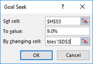
Then we click [OK] and that find cash receipts from landscaping services must increase to $30,010 to earn an ROE of 9%. Furthermore, increasing cash receipts from landscaping services to $30,010 increases total cash receipts to $39,000. Changes in the endogenous variables included in system are described next in the activity column of the what if page.
Table 6.5. What If Analysis
using SPELL Ratios.
Open Table 6.5 in Microsoft Excel
| Ratios | Industry Average | Activity Ratios | HQN Base | Goal Seek |
| Solvency | ||||
| TIE | 2.50 | 1.38 | 1.35 | 1.38 |
| DSR | 1.40 | 1.03 | 1.02 | 1.03 |
| Profitability | ||||
| ROA | 3.30% | 6.60% | 6.50% | 6.60% |
| ROE | 10.70% | 9.00% | 8.50% | 9.00% |
| m margin | 29.00% | 0.45% | 0.43% | 0.45% |
| Efficiency | ||||
| ITO | 7.7 | 10.67 | 10.67 | 10.67 |
| ITOT | 47.4 | 34.21 | 34.22 | 34.21 |
| ATO | 3.2 | 4.00 | 4.00 | 4.00 |
| ATOT | 114.1 | 91.23 | 91.25 | 91.23 |
| RTO | 11.41 | 24.40 | 24.39 | 24.40 |
| RTOT | 32 | 14.96 | 14.97 | 14.96 |
| PTO | 12.59 | 9.33 | 9.33 | 9.33 |
| PTOT | 29 | 39.11 | 39.12 | 39.12 |
| Liquidity | ||||
| Current Ratio | 1.30 | 1.06 | 1.06 | 1.06 |
| Quick Ratio | 0.70 | 0.43 | 0.43 | 0.43 |
| Leverage | ||||
| Debt/Assets | 0.91 | 0.80 | 0.80 | 0.80 |
| Debt/Equity | 2.00 | 4.00 | 4.00 | 4..00 |
| Asset/Equity | 2.20 | 5.00 | 5.00 | 5.00 |
Note that increasing CR from landscaping services to $39,000 resulted in an increase of ROE to 9.00%. Of course, there were other consequences. ROA increased to 6.6%. The TIE solvency ratio increased slightly from 1.35 to 1.38. These and other changes we observe by comparing the activity and goal seek columns with the HQN base column.
Creating Subsystems
It is important to be able to answer what if and how much questions, especially about such important endogenous variables as ROE in a smaller system than the CFS. We create subsystems by redefining the boundaries between exogenous and endogenous variables in the system.
To simplify the connections between exogenous and endogenous variables in systems, we define subsystems and ask what if and how much questions about the subsystems. We create a subsystem by redefining some endogenous variables in the system as exogenous variables. This permits us to examine the consequences of particular shocks on a reduced number of particularly interesting endogenous variables.
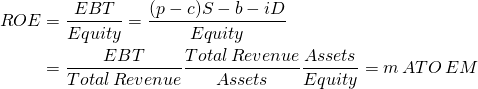
We can construct a large number of subsystems. However, we focus on the two subsystems that matter most to the firm: those that describe the firm’s ROE and its solvency. To illustrate, suppose we wanted to build a subsystem around the firm’s ROE. Letting letters represent system endogenous variables, we might begin by assuming that the firm sells each item of what it produces at an exogenously determined price p, that its marginal cost is c, its fixed overhead expenses (OE) cost is b, and that its interest costs are iD where i is the average cost of its debt and D is the sum of the firm’s liabilities determined in the previous period. Finally, letting the number of physical units sold equal S, we define our ROE subsystem by assuming all other variables except ROE to be exogenous. We have now created an ROE simplified subsystem. We define Earning Before Taxes (EBT) in the subsystem as:
(6.1)

Now we can write the ROE subsystem as:
(6.2)
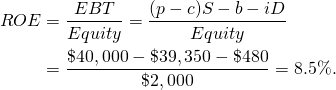
Having defined an ROE subsystem, we are prepared to ask what if questions such as: what would happen to the firm’s ROE if we could increase the ATO by increasing cash receipts? Since our subsystem has defined all of the interdependencies, we can find the answer to this what if question by observing the change in the firm’s ROE in response to changes in the system’s exogenous variables. We illustrate the approach using HQN’s data. Initially, HQN’s ROE equals:
(6.3)
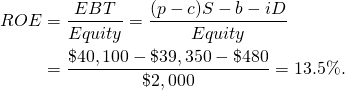
Suppose the value of the exogenous variable cash receipts increased to $40,100? The results on the firm’s ROE can be found to equal:
(6.4)
Another subsystem might involve solvency and the TIE ratio. To analyze this subsystem, we begin with the simplified EBT subsystem defined earlier and remove interest costs to obtain earnings before interest and taxes (EBIT) equal to:
(6.5)

Next we write a DuPont type equation focused on TIE equal to:
(6.6)

where DE is the debt-equity leverage ratio. Having now defined a solvency subsystem reflected by the firm’s TIE ratio, we can ask the following what if question. What if the firm increased its debt D? Then, what would be the effect on the firm’s solvency? To answer this what if question, we substitute the simplified EBIT formula into Equation \ref{6.10} to obtain:
(6.7)

To illustrate, we substitute HQN’s data into Equation \ref{6.11} to find its initial TIE value. Making the substitution we find:
(6.8)

Now suppose we ask: what if the firm’s equity falls by $1,000? In response to this change in an exogenous variable, HQN’s TIE ratio would decline to:
(6.9)
And what if the firm’s interest rate increased by one percent to 7.0%? Then its TIE ratio becomes:
(6.10)
It is important to recognize that the answers to our what if questions answered in our subsystems are only approximations of what would happen if we considered the entire system. Nevertheless, the subsystem approach provides some useful intuitive explanations that may be disguised in a full system analysis.
Common Size Balance Sheets and Common Size Income Statements
When comparing financial statements across time and across firms, it is often useful to standardize the statements. The typical way this is done is by expressing all items in the balance sheet as a percentage of total assets and all items in the income statement as a percentage of total revenue. Common size balance sheets and common size income statements facilitate comparison across time and across firms because absolute size effects are eliminated by expressing numbers in the statements as percentages of the same whole.
One of the significant advantages of common size balance sheets and common size income statements is that they allow all items in either the balance sheet or income statement to be compared to an industry standard. There is one other thing, however, that happens when we convert balance sheets and income statements to ratios reflecting a percentage of the whole: all the variables in the statements become interdependent—an increase in one variable requires decreases in other variables in the statements because their sum must equal 100%. Furthermore, this requirement that they sum to 100% creates a type of closed system in which all the entries except one sum to 100%. This enables us to do trade-off analysis.
Consider what we can learn from common size balance sheet statements. Suppose that a firm’s cash position was $100,000 at the end of 2017 and $110,000 at the end of 2018. In addition, suppose the firm’s total assets were $2,000,000 at the end of 2017 and $3,000,000 at the end of 2018. The absolute value of the firm’s cash position increased by $10,000 over the year which might suggest the firm is now more liquid. However, the firm’s cash position must now support a larger amount of total assets. Looking at the cash position as a percentage of total assets, we find the firm’s cash position was 5% of total assets at the end of 2017, and only 3.67% at the end of 2018. Thus, the amount of cash available per dollar of assets held by the firm actually decreased during the year. Common size balance sheets for HQN are presented in Table 6.7.
Table 6.6. Common Size Balance Sheets for HQN
| 2016 | 2017 | 2018 | Ind. Ave. | |
| ASSETS | ||||
| Cash and Marketable Securities | 12.13% | 9.30% | 5.77% | 6.3% |
| Accounts Receivable | 15.77% | 16.40% | 11.54% | 26.4% |
| Inventory | 31.85% | 37.50% | 50.00% | 25.6% |
| CURRENT ASSETS | 59.76% | 63.20% | 67.31% | 58.3% |
| Depreciable long-term assets | 33.06% | 29.90% | 26.92% | 35.7% |
| Non-depreciable long-term assets | 7.18% | 6.90% | 5.77% | 6.0% |
| LONG-TERM ASSETS | 40.24% | 36.80% | 32.69% | 41.7% |
| TOTAL ASSETS | 100.00% | 100.00% | 100.00% | 100.00% |
| LIABILITIES | ||||
| Notes Payable | 4.16% | 15.00% | 12.21% | 13.9% |
| Current Portion LTD | 7.085% | 5.00% | 4.33% | 3.6% |
| Accounts Payable | 24.27% | 30.00% | 38.46% | 18.7% |
| Accrued Liabilities | 8.80% | 9.58% | 8.46% | 6.8% |
| CURRENT LIABILITIES | 54.30% | 59.58% | 63.46% | 43.0% |
| NON-CURRENT LONG-TERM DEBT | 25.88% | 20.42% | 19.09% | 13.4% |
| TOTAL LIABILITIES | 80.18% | 80.00% | 82.55% | 56.4% |
| Equity | 19.82% | 20.00% | 17.45% | 43.6% |
| TOTAL EQUITY | 19.82% | 20.00% | 17.45% | 43.6% |
| TOTAL DEBT AND EQUITY | 100.00% | 100.00% | 100.00% | 100.00% |
Entries in HQN’s common size balance sheet can be examined by comparing them with other firms in the industry described in the last column of Table 6.7. HQN’s level of current assets is above the industry average and rising, primarily as a result of relatively high and increasing inventory levels. The accounts receivable levels are low in terms of the industry levels. Long-term asset levels are also low, relative to industry levels, and declining. Current liabilities are well above the average levels in the industry, and rising mostly as a result of increasingly high levels of accounts payable. Although falling, long-term debt is still above industry averages. Owner equity levels are well below the average firm in the industry.
Common size income statements. Entries in HQN’s common size income statement can be examined by comparing them with other firms in the industry described in the last column of Table 6.8. Consider what we might learn from HQN’s common size income statements. HQN’s cost of goods sold (COGS) as a percentage of cash receipts in 2018 was close to the industry average. However, its overhead expenses (OE) were much higher than the industry average in both 2017 and 2018. As a result, its EBIT as a percent of cash receipts was much lower than the industry average. Furthermore, its interest costs as a percentage of cash receipts were almost double the industry average. HQN’s high OE and high interest costs relative to the industry were somewhat mitigated by HQN’s lower than industry standards depreciation and taxes. Still, HQN’s net income after taxes (NIAT) as a percentage of cash receipts in 2018 is low compared to the industry average: 0.25% for HQN versus 2.28% for the industry.
“What if” questions and the common size financial statements. Common size balance financial statements are derived from the CFS. As a result they respond to changes in endogenous and exogenous variables that make up the common size financial statements. Furthermore, we can ask what if and how much kinds of questions of the CFS and observe their changes in the common size financial statements.
For example, suppose that HQN’s cash receipts increased from $38,000 in 2017 to $40,000 in 2018. Meanwhile, suppose its COGS increased from $25,600 to $28,000. We may want to know if COGS increased in proportion to its increased cash receipts. From the common size income statement we see that as a proportion of its cash receipts, COGS increased from 67.37% in 2017 to 70% in 2018, suggesting that its COGS increased at a rate greater than its cash receipts—a result that should concern the financial manager.
Table 6.7. Accrued Common Size Income Statements for HQN
| 2017 | 2018 | Ind. Ave. | |
| Total Revenue | 100.00% | 100.00% | 100.00% |
| Cost of Goods Sold (COGS) | 67.37% | 70.00% | 71.40% |
| Overhead Expenses | 29.82% | 27.50% | 22.50% |
| Depreciation | 1.24% | 0.88% | 1.75% |
| EARNING BEFORE INTEREST AND TAXES (EBIT) | 1.58% | 1.62% | 4.35% |
| Interest | 1.22% | 1.20% | 0.55% |
| EARNINGS BEFORE TAXES (EBT) | 0.36% | 0.42% | 3.80% |
| Taxes | 0.17% | 0.17% | 1.52% |
| NET INCOME AFTER TAXES (NIAT) | 0.19% | 0.25% | 2.28% |
Common Size Statements and Trade-offs
That entries in common size statements sum to 100% means that we cannot increase one variable in the statements without decreasing another variable in the statement. Therefore, any change in an exogenous variable that affects the proportion of that variable in the common size statement will have some offsetting impact on at least one other variable in the system. We may refer to these cause-and-effect changes in exogenous variables as trade-offs. There are various ways we can describe these trade-offs.
The Squeeze versus the Bulge. One way to examine trade-offs is to assume the financial system has some characteristics similar to a balloon. If a squeeze happens somewhere on the balloon, a corresponding bulge will occur somewhere else—because balloons require equal pressure on its surface. This balloon-like characteristic is evident in common size financial statements.
For example, suppose the firm wishes to increase its liquidity and so increases the percentage of its assets held as accounts receivable. However, if the percent of assets must add to 100%, increasing the percentage of short-term assets will require that the percentage of long-term assets decrease—and profitability and perhaps efficiency suffers.
CFS and trade-offs. Trade-offs are obvious within common size statements. They exist within the CFS system but may be less obvious. Some usual trade-offs are summarized in the table the follows. Consider the left-hand column as the “squeeze” and the right-hand column is a possible “bulge.” However, the “squeeze” and “bulge” comparisons described below are only qualitative possibilities. To find out the quantitative connections, we must look at the firm’s ratios and common size statements. Still, the principle is important: when analyzing the firm by examining a particular ratio, look for its companion ratio.
Table 6.8. The Squeeze vs. The Bulge
| The Squeeze | The Bulge |
| leverage ratio (D/E): High | rate of return on equity (ROE): High |
| cash receipts/inventory ratio (ITO): High | cash receipts/accounts receivable (RTO): Low |
| cash receipts/inventory ratio (ITO): Low | profit margin (m): Low |
| current assets/current liabilities ratio (CR): High | rate of return on equity (ROE): Low |
| cash receipts/assets ratio (ATO): High | operating and repair: High |
| COGS/notes payable (PTO): High | interest costs: High |
Companion ratios. We apply the principle of looking for interesting things in pairs to HQN. Is anything else unusual about HQN? Yes! Look at its inventories in the common size balance sheet: 50% of its assets in 2018 versus an industry average of 25.6%. We have found a squeeze. The bulge? Look at accounts receivable: 11.54% versus an industry standard of 26.4%. Does this suggest that the firm has adopted a stringent credit policy that has discouraged customers? Perhaps. It’s an area the firm should likely explore. If HQN’s stringent credit policy were indeed affecting cash receipts, then its inventory turnover ratio (ITO) would be affected, but this ratio isn’t too far out of the ordinary: 10.67% versus the industry median of 7.7%. However, the upper quartile for the industry is 14.9%, suggesting a large variability for the industry. So, the firm’s credit policy is not off the hook yet.
Anything else unusual about HQN? Well, yes. Its debt to equity ratio is 4.0 in 2018 versus the industry average of 1.9. Unfortunately for HQN, a high leverage ratio hasn’t increased profits or rates of return as much as might be expected because of its low efficiency and possibly an ineffective cash receipts strategy. Continuing, if HQN has unusually high levels of debt relative to its equity, we should expect its interest payments to be above the industry average. They are 1.2% of cash receipts in 2018 versus an industry average of .55%. Already we are alarmed; high leverage is usually accompanied by high risk. One reason that high leverage implies high risk is that the firm’s equity relative to its liability is small, and not able to handle and survive a market reversal. Is HQN’s equity low relative to the industry? Very much so: 17.45% in 2018 versus the industry average of 43.6%.
Trend Analysis
Using historical data, we attempt to look ahead to financial conditions likely to be experienced in the future. Consider the common size balance sheets reported earlier in Table 6.7. The first step is to look for any significant changes or trends in the asset or liability accounts. Current assets have increased over the three year period mostly due to a significant increase in inventory levels. Cash levels declined during the three years for the same reason—current assets being tied up in inventory. Long-term assets have fallen primarily as a result of declining values of the firm’s property, plant, and equipment. The worrisome result of this trend is that it may project increased maintenance costs associated with aging machinery.
On the debt side of the balance sheet, current liabilities have increased during the three year period mostly as a result of increases in accounts payable. Long-term debt has declined, and owner equity has remained relatively constant. The question associated with this trend is, can increasing dependence on notes payable be sustained? Are there less expensive sources of financing available?
Examining HQN’s common size income statement, reported in Table 6.8, we see that both EBIT and NIAT increased in 2018 as a percentage of cash receipts. Comparing HQN’s income statement with other firms in the industry, we note that HQN’s EBIT and NIAT were low compared to industry averages, primarily as a result of relatively high overhead expenses and interest expenses. High OE, COGS, and interest costs have reduced HQN’s taxes.
The statement of cash flow in Table 6.9 confirms that cash levels in the firm have been declining. However, cash flow from operations was positive in both 2017 and 2018. The firm had positive income and additional cash flow was generated by depreciation expense and increases in current liabilities. A large cash inflow was also received in 2017 as a result of a decrease in accounts receivable. One salient point is that the firm sacrificed significant amounts of cash in 2017 and 2018 to increase inventory levels.
Table 6.9. HQN’s Coordinated Financial Statements for Year 2018 after a cash receipts change in an exogenous variable
| BALANCE SHEET | ACCRUAL INCOME STATEMENT | STATEMENT OF CASH FLOW | ||||||
| DATE | 12/31/2017 | 12/31/2018 | DATE | 2018 | DATE | 2018 | ||
| ASSETS | + | Cash Receipts | $39,990 | + | Cash Receipts | $39,990 | ||
| Cash and Marketable Securities | $930 | $1,600 | + | Change in Accounts Receivable | ($440) | – | Cash Cost of Goods Sold | $27,000 |
| Accounts Receivable | $1,640 | $1,200 | + | Change in Inventories | $1,450 | – | Cash Overhead Expenses | $11,078 |
| Inventory | $3,750 | $5,200 | + | Realized Cap. Gains/Depr. Recapture | $0 | – | Interest paid | $480 |
| Current Assets | $6,320 | $7,000 | Total Revenue | $41,000 | – | Taxes | $68 | |
| Property, Plant, and Equipment | $2,990 | $2,800 | + | Cash Cost of Goods Sold | $27,000 | Net Cash Flow from Operations | $1,364 | |
| Other Assets | $690 | $600 | + | Change in Accounts. Payable | $1,000 | + | Realized Cap. Gains + Depr. Recapture | $0 |
| Long-Term Assets | $3,680 | $3,400 | + | Cash Overhead Expenses | $11,078 | + | Sales Non-depreciable Assets | $0 |
| TOTAL ASSETS | $10,000 | $11,400 | + | Change in Accrued Liabilities | ($78) | – | Purchases Non-depreciable Assets | |
| LIABILITIES | + | Depreciation | $350 | + | Sale Depreciable Assets | $30 | ||
| Notes Payable | $1,500 | $1,270 | Total Expenses | $39,350 | – | Purchases Depreciable Assets | $100 | |
| Current Portion Long-Term Debt | $500 | $450 | Earnings Before Interest and Taxes (EBIT) | $1,650 | Net Cash Flow from Investment | ($70) | ||
| Accounts Payable | $3,000 | $4,000 | – | Less Interest Costs | $480 | + | Change in Non-Current Long Term Debt | ($57) |
| Accrued Liabilities | $958 | $880 | Earnings Before Taxes (EBT) | $1,170 | + | Change in Current Portion of Long Term Debt | ($50) | |
| Total Current Liabilities | $5,958 | $6,600 | – | Less Taxes | $68 | + | Change in Notes Payable | ($230) |
| Non-Current Long Term Debt | $2,042 | $1,985 | Net Income After Taxes (NIAT) | $1,102 | – | Less Dividends and Owner Draw | $287 | |
| Contributed Capital | $1,900 | $1,900 | – | Less Dividends and Owner Draw | $287 | Net Cash Flow from Financing | ($624) | |
| Retained Earnings | $100 | $915 | Addition to Retained Earnings | $815 | CHANGE IN CASH POSITION | $670 | ||
| Total Equity | $2,000 | $2,815 | ||||||
| TOTAL LIABILITIES AND EQUITY | $10,000 | $11,400 | ||||||
Cash was used each year to increase investments in long-term assets. However, the amount of assets used each year was significantly greater than the amount reinvested in long-term assets. For example, in 2018 the firm used up $350 in assets (the amount of depreciation expense) and only had a net investment of $70,000, a depletion of $280,000 in the firm’s assets.
Cash was also used each year in the firm’s financing activities. The firm made a large payment of long-term debt in 2017. Then in 2018, a large equity withdrawal was made. Both of the payments were larger than the cash flow produced out of the firm’s operations.
Common Size Statements and Pro Forma Financial Statements
Consider how financial managers can use financial ratios to forecast the financial condition of the firm by asking what if questions whose answers produce pro forma balance sheet and income statements. Financial forecasting is a method used by firms to help plan for future financial needs. However, using pro forma income statements and pro forma balance sheets both require that each one is defined as a subsystem.
Pro forma income statements and balance sheets are forecasts of what these statements will look like in the future and provide essential planning information. There are several ways to construct pro forma statements. The usual technique is to select a key variable and predict its future value. Then assume constant SPELL ratios which include the key variable and solve for other values using other ratios. We demonstrate this approach in what follows.
Assume that HQN wants to achieve a projected level of cash receipts. Also assume that SPELL ratios will remain constant even in the face of projected total revenue increases. Specifically, assume that next year’s projected total revenue for HQN will equal $42,000, an increase of 5%. What does this imply for HQN’s level of inventory? From HQN’s financial ratios, we see that the inventory turnover ratio was 10.67%. Assuming that this year’s ratios will hold next year, we can use the projected level of cash receipts to forecast the pro forma levels of inventories (INV). The first step in these types of problems is to write out the definition of each ratio and their assumed values:
(6.11)
From the inventory turnover (ITO) equation we find:
(6.12)

Next we use the projected cash receipts level of $42,000 and divide by ITO to find projected HQN’s inventory in 2019:
(6.13)

But now, we observe an interesting result, inventory increased by 5% to $4,038.46, the same percentage increases as was projected in total revenue. This result, of equal percentage increases, occurs whenever the ratio is held fixed. When one number of the ratio is increased by some percent, the other number in the ratio must increase by the same percent. To illustrate, consider the m ratio:
(6.14)
If the m ratio is constant and cash receipts increases to $42,000, then EBIT will increase by 5% to $178.50. Again, the technique is to assume that the historical financial relationships will hold in the future and then project the future value of one variable, usually cash receipts. This allows us to calculate the projected values of the remaining financial variables based on the historical financial relationships. Of course, we could create pro forma income statements and balance sheets by increasing all the variables by some common percent, or just the exogenous variables by the common percent. However, increasing all the exogenous variables by a common percent is confusing, and it is highly unrealistic. Instead, we will suggest the change in an exogenous variable analysis approach described next.
Summary and Conclusions
We began this chapter by describing the CFS as a system in which changes in one part of the system affected other parts of the system. We reminded ourselves that while ratios can describe the firm’s strengths and weaknesses, they cannot answer what if and how much kinds of questions unless they are embedded in a system.
Then, we faced the fact that the world is a really complicated system and we can’t learn much about it without creating subsystems that assume or define some endogenous variables as exogenous variables. In effect, we create subsystems from systems by reducing the number of endogenous variables and increasing the number of exogenous variables—allowing us to describe a subsystem within a system with a reduced number of endogenous variables.
We found our subsystems to be useful because they allow us to understand the connections between some of the most important parts of the financial system, such as its rates of return and its solvency. While there are a large number of subsystems we could create and examine, we emphasized the firm’s TIE ratio and its ROE ratios.
Another important concept emphasized in this chapter was that the nature of the system implies that changes in exogenous variables produce consequences on more than one endogenous variable, and these changes in more than one endogenous variable can be described as trade-offs. Trade-offs are one way to answer what if questions. For example, what if the changes in an exogenous variable were increased cash receipts? Then what is the effect on COGS, ROE, or other endogenous system variables? Several of these important trade-offs were described in this chapter. We also answered how much questions with the help of Excel’s goal seek. How much questions help us find the requirements for reaching specific financial goals.
Finally, we recommended that we examine changes in exogenous variables in the context of the CFS system. And to practice, we suggested learners consider several scenarios. One way to practice finding the impacts of change in an exogenous variable was an exercise we referred to as what if analysis or how much analysis. This chapter provided several scenarios that could be examined using what if and how much analysis—which is the essence of opportunities and threats analysis.
Questions
- Describe a system, one that is different than the financial system described in this chapter.
- In this chapter, we treated taxes as an exogenous variable in the CFS system. Describe how you would convert taxes from being an exogenous variable to an endogenous variable.
- Perform a what if analysis by describing how an increase in NIAT would influence other endogenous variables in the CFS system.
- Refer to Table 6.9. Then, list the endogenous and exogenous variables in the end of period Balance Sheets, the Income Statement, and the Statement of Cash Flow.
- Compare HQN’s common size balance sheet at the end of years 2016, 2017, and 2018. Notice that cash and marketable securities were well above the industry average in 2016 and then declined in both 2017 and 2018 to a level below the industry average. By referring to other ratios in the common size balance sheet, explain what changes in the firm likely account for HQN’s decline in liquidity.
- Refer to Table 6.1. Then, observe that HQN’s account receivables declined from 2017 to 2018. What effect did this decline have on HQN’s liquidity? What effect did the decline have on the firm’s cash and marketable securities?
- Refer to Table 6.1. Then, observe that HQN’s current liabilities increased from 59.58% in 2017 to 63.46% in 2018. In all years, current liabilities were well above the industry average of 43%. What changes at HQN’s may account for the rise in current liabilities as a percentage of total assets? Is this change a strength or weakness of the firm? Provide a possible explanation for the HQN’s change in its current liabilities.
- Focusing on HQN’s common size income statement in Table 6.7, observe that overhead expenses were increasing between 2017 and 2018 while depreciation was low. Are the two connected? Can you connect this change to changes in the firm’s long-term assets in the common size balance sheets?
- The common size income statement’s base is cash receipts. Recalculate the common size income statements for 2017 and 2018 using COGS as the new base. What is the effect of changing the base in the calculation of the common size income statement?
- In Table 6.7, NIAT is especially low compared to the industry average. Can you explain why?
- Choose three of the ten scenarios described in the text. Then do the following opportunities and threats procedures. First, perform a what if exercise that includes the following steps. Use the Excel worksheet supplied in class and perform what if and how much exercises consistent with the conditions described in the scenario. Identify the responses to the changes in an exogenous variable in financial statements. Recognize that some connections may require more than one exogenous variable be changed. Then recalculate the affected ratios and the common size balance sheet and income statements. Finally, write a brief opportunities and threats report about how the conditions described in the scenario would change the firm’s opportunities and threats.
- Compare HQN’s 2017 and 2018 common size balance sheet in Table 6.6 with the industry average. Based on these comparisons, what are some financial strengths and weaknesses of HQN compared to the industry?
- Compute a pro forma income statement for HQN for 2019. Assume cash receipts equals $42,000 and the relationships described by the common size income statement for 2018 are maintained.