
14: Homogeneous Liquidity
- Page ID
- 12759

After completing this chapter, you should be able to: 1. Learn how to measure an investment’s liquidity. 2. Learn how to compare liquidity for a firm versus liquidity for an investment. 3. Learn how to rank investments according to their liquidity using cash flow measures.
To achieve your learning goals, you should complete the following objectives:
- Learn to distinguish between two types of returns earned by an investment: time dated cash flow and capital gains (losses).
- Learn how to distinguish between a firm’s liquidity and an investment’s liquidity.
- Learn how to describe an investment’s liquidity at a point in time by using its current-to-total returns (CTR) ratio.
- Learn how to describe an investment’s liquidity over time by using its inter temporal CTR ratio.
- Learn how to connect CTR ratios to price-to-earnings (PE) ratios.
- Learn how PE ratios can be used to infer the liquidity of an investment.
- Learn how coverage (C) ratios can be used to infer the liquidity of an investment.
Introduction
An investment may earn two types of returns (losses) for investors: (1) time-dated cash flow called current returns, and (2) capital gains (losses). This chapter demonstrates that capital gains earned on an investment depend on the investment’s pattern of future cash flow.
This chapter also demonstrates that the combination of current returns versus capital gains (losses) has important liquidity implications for investors, especially when an investment is financed with debt capital. Debt-financed investments whose earnings are expected to grow over time may experience a cash shortfall called a financing gap, in which the cash returns are less than the scheduled payments of principal plus interest. This gap is most likely to occur early in the investment’s life and is exacerbated by inflation. As time passes and the cash returns grow in size, they will eventually exceed the repayment obligation, and the liquidity problem is solved.
The term liquidity is used to describe “near-cash investments” because of the similarity between liquids and liquid investments. A liquid such as water can fill the shape of its container and is easily transferred from one container to another. Similarly, liquid funds easily meet the immediate financial needs of their owners. Illiquid investments such as land and buildings, like solids, are not easily accessed to meet financial needs because their ownership and control are not easily transferred.
A firm’s liquidity reflects its capacity to generate sufficient cash to meet its financial commitments as they come due. A firm’s failure to meet its financial commitments results in bankruptcy, even though the firm might be profitable and have positive equity. Consequently, firms must account for an investment’s liquidity in addition to earning positive net present value (NPV).
There are several measures that reflect a firm’s or an investment’s liquidity. One measure used to reflect the liquidity of the firm is the current ratio, the ratio of current assets divided by current liabilities. Because current assets can be quickly converted to cash, they are an important source of liquidity for the firm.
While the current ratio measures the liquidity of the firm, we want a liquidity measure specific to an investment, and one that describes the liquidity of an investment over time—what we will refer to as a periodic liquidity measure. The liquidity measure that provides investment-specific liquidity information over time is the current-to-total returns (CTR) ratio. The CTR ratio is derived from market equilibrium conditions where NPV is zero and represents the ratio of current (cash) returns to total returns. The price-to-earnings (PE) ratio is a commonly reported ratio reflecting the price of an investment reflected by its current earnings. A liquidity measure related to the CTR ratio is the coverage (C) ratio. A C ratio is the ratio of cash returns to loan payments or other debt obligations in any particular period.
Current-to-Total-Returns (CTR) Ratio
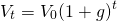
The current-to-total returns (CTR) ratio is a periodic liquidity measure derived from the relationship in a given period between an investment’s current (cash) returns, its capital gains (losses), and its total return, or the sum of current returns and capital gains (losses). To derive the CTR measure, we begin with an expression of an investment’s total returns:
Total investment returns = current returns + capital gains (losses)
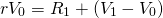
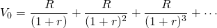
The above relationship is expressed symbolically as follows. Let the investment’s total return equal the investment’s internal rate of return r times the value of the investment at the beginning of the period V0 or rV0. Meanwhile, let R1 be defined as the asset’s net cash, or current returns earned at the end of the first period. In addition, let V0 and V1 equal the investment’s beginning and end-of-period values respectively, while their difference (V1 – V0) is equal to the investment’s capital gains (losses) in the first period. Summarizing, we write the investment’s total returns as:
(14.1)
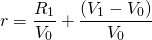
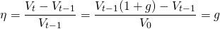
Next we solve for the investment’s internal rate of return earned in each period, r. We solve for this measure by dividing the investment’s total returns by the investment’s value at the beginning of the period V0:
(14.2)
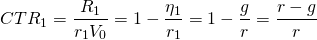
A useful measure obtained from Equation \ref{14.2} is the ratio of current returns R1 divided by total returns rV0. This ratio indicates the percentage of total returns the firm receives as cash. The higher this ratio, the greater the likelihood that the firm has the liquidity required to meet its debt obligations in the current period. Rearranging the previous equation yields the ratio of current to total returns in the first period, equal to CTR1:
(14.3)
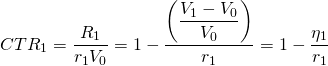
where  is the capital gains (loss) rate in period one.
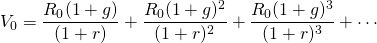
To illustrate the CTR ratio, we now derive the CTR ratio for the geometric series of cash flow. Consider an investment that is expected to generate a perpetual series of cash flow that grow at average geometric rate of g percent per period. If R0 is the initial net cash flow, and r is the IRR of the investment, then the PV of the growth model can be expressed as:
(14.4a)
One year later:
(14.4b)

and in general
(14.4c)
and the capital gains rate for the geometric growth model is found to equal:
(14.4d)
Using our results from Equation \ref{14.3} we can find our CTR ratio as:
(14.5)
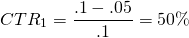
To illustrate, if an investment earns cash flow in perpetuity described by R0, r = 10% and g = 5%, the investment’s CTR ratio can be found equal to:
(14.6)
It is left as an exercise to demonstrate that if the CTR ratio is constant over time, the CTR ratio is 1. Namely, that:
(14.7a)
To illustrate equation (14.7a), if in period one, r = 10% and g = 5%, then 50% of the investment’s returns will be earned in the form of capital gains. On the other hand, if the geometric mean of changes in future cash flow was negative, (g < 0), the current returns to total returns would exceed total returns. If g = –5%, the CTR1 ratio would equal:
(14.7b)
In words, equation (14.7b) informs us that 150% of the investment’s return in period one will be received as current returns in order to compensate for the 50% capital losses experienced by the investment.
Liquidity, Inflation, and Real Interest Rates
Prices reflect the ratio of money exchanged for a unit of a good. For example, assume that the price for gasoline is $3.00 per gallon. If you purchased 10 gallons of gasoline, you would pay $30.00 ($3.00 x 10). Conversely, the ratio of $30.00 expended for gas divided by the gallons of gas purchased is the price of gas: $30.00/10 equal to $3.00.
Now suppose that last year you purchased roughly
$50,000 worth of goods. For convenience, let pj
be the price of good j where j = 1, …,
n. Furthermore, let qj represent the
quantity of good j purchased. Multiplying the price times
the quantity of each good purchased equals your total expenditures
of $50,000. To summarize,  equals the sum of price times quantity of all of the goods you
purchased.
equals the sum of price times quantity of all of the goods you
purchased.
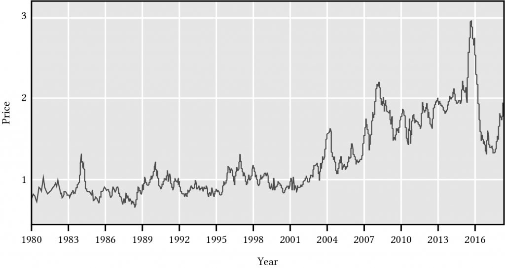
In case you had not noticed, prices for goods and services change over time. Consider the price of a dozen large eggs. The price of a dozen of large eggs over the past 38 years is graphed in Figure 14.1 ranging from less than $1 per dozen in 1980 to almost $3 per dozen in 2016.
Figure 14.1. The price of a
dozen large eggs over the period 1980 to 2016.
(Bureau of Labor Statistics, 2016)
Prices over time for an individual good can change for several reasons. The demand for eggs can rise—more people wanting to consume more eggs will likely cause egg prices to rise. Or the cost of supplying eggs may change—chicken have become more efficient at producing eggs making them cheaper or chicken feed may become more expensive making eggs more expensive to produce.
The quantity theory of money
There is another reason why prices may change over time—there is more money in circulation. This explanation for why prices rise we call the quantity theory of money (QTM). The quantity theory of money states that there is a direct relationship between the quantity of money in an economy and the level of prices of goods and services sold. What constitutes the money supply is a complicated subject that we can avoid here and still make our point.
Returning to our earlier discussion, let the total of goods and services sold times their prices equal the amount of money M in the economy times its velocity (V) or the number of times the same unit of money is used during a time period. We write this relationship as
(14.8)
According to the QTM, if people purchased the same goods in the same quantity and if V were held constant and M increased by i percent, then the price of each individual good must also increase by i percent.
(14.9)
Finally, if we measured the prices times the same goods in each year and calculated the ratio of the current year by the previous year we could obtain an estimate of the how prices in general have changed or the rate of inflation. Adding a superscript t to the price variable, we find the inflation rate plus one in year t is equal to:
(14.10)
An index (1 + i) can be computed for all different bundles of purchased goods. One popular inflation index is called the Consumer Price Index (CPI) that measures the rate of increase in prices holding the bundle of goods constant or at least as far as it is possible. Consider how inflation has affected consumer purchases over time. The vertical axis measures the CPI. The horizontal axis measures time. All indices select one year at their base in which the index is one. In Figure 14.2, the base year is somewhere between 1982-1984.
Figure 14.2. The consumer price index for all the U.S. letting average prices between 1982-84 equal 100.
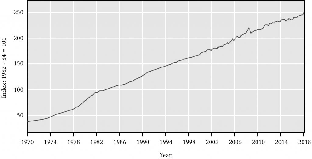
According to Figure 14.2, in 2018 you paid on average two and one-half times as much money to purchase the same good as you did in 1982-1984.
So why is inflation important to our discussion of PV models and profit measures? If your income increases by i percent and the cost of everything you purchase increases by the same percent i, then in real terms what you can actually purchase is the same as before since your income and costs increased by the same rate.
Real interest rates. Let say that your after-tax cash flows increased by rate g% but that g is influenced by the rate of inflation. Then after accounting for inflation, what is left is attributed to other factors besides an increase in the money supply. Let this real growth in after-tax cash flow (ATCF) be g*. Then we can write:
(14.11)
Interest rates, discount rates, and inflation. Inflation also influences interest rates paid to borrow money and the discount rate that reflects the opportunity cost for one’s resources. To motivate this discussion intuitively, assume you lent a friend $1000 for one year. Also assume that inflation is 5% so that when your friends repays the loan, to make the same purchases at the time the loan was made, they would have to pay back $1,000 * (1.05) = $1,050. But they would have to pay more than 5% for being able to rent your money for a year—let’s call this rate the real interest rate and denote it as r*. To account for both the reduced purchase price of your money because an increase in prices by inflation i and the cost of postponing the use of one’s money, the interest rate (and opportunity cost of resources invested in a defender) is r equal to:
(14.12)
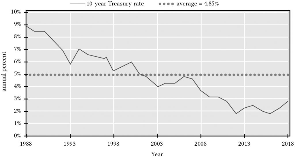
We graph real interest rates r* over time in Figure 14.3.
Figure 14.3. 10-year Treasury constant maturity interest rate, U.S., 1988 – 2018
Liquidity Implications
The mix of capital gains (losses) versus current returns depends directly on the average rate of growth (g > 0) or decline (g < 0) in future cash flow. As inflation increases the average rate of growth g, then inflation also reduces an investment’s liquidity, especially during the investment’s initial years.
For geometric decay in earnings (g < 0), current returns are more than 100% of total earnings—and current returns have increased in importance relative to capital loss or depreciation. These results clearly show the paradoxical conditions that growth in projected earnings can weaken the liquidity of the investment due to the increasing relative importance of capital gains. In contrast, a decline in projected earnings can strengthen the liquidity due to the increasing relative importance of current returns (See Table 14.1).
Also note in Table 14.1 that increases in the capital gains rate g holding r constant always leads to a reduction in CTR ratio. This is easily explained. Since the total rate of return r is fixed and composed of current rate of returns and capital gains rate of returns, increases in the capital gains rate of return must necessarily decrease the current rate of returns.
Table 14.1. Values of CTR ratios where CTRt = (r – g) / r
| r% | |||||
| g% | 10 | 8 | 6 | 4 | 2 |
| –5 | 150% | 163% | 183% | 225% | 350% |
| –3 | 130% | 138% | 150% | 175% | 250% |
| 0 | 100% | 100% | 100% | 100% | 100% |
| 3 | 70% | 63% | 50% | 25% | |
| 5 | 50% | 38% | 17% | ||
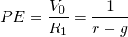
Price-to-earnings (PE) Ratios
Related to the CTR ratio is the price-to-earnings (PE) ratio equal to:
(14.13)

If we describe the investment using the PV expression in equation (14.4a), then we can write:
(14.14)

Next we substitute R0(1 + g) for R1, and the right-hand side of Equation \ref{14.9} for V0 into the PE expression in Equation \ref{14.8}, and obtain:
(14.15)
But from equation (14.7a) we know that rCTR = (r – g), which allows us to connect CTR and PE ratios, namely:
(14.16)

In words, what we learn from Equation \ref{14.16} is that, in general, higher CTR ratios imply lower PE ratios and lower CTR ratios imply higher PE ratios. These results may at first appear to be somewhat counter intuitive—that, for liquidity purposes, we prefer investments with lower PE. Upon reflection, it makes sense—assets whose returns are mostly capital gains will be earning a lower percentage of current returns compared to their values than assets that earn little or no capital gains.
To make the point that CTR and PE ratios are inversely related, we construct Table 14.2 for PE ratios. Compare the results with those found in Table 14.1 to confirm in your minds the implications of Equation \ref{14.16}. Note that PE ratios uniformly increase with increases in g and the rate of return earned in the form of capital gains.
Table 14.2. Values of PE ratios where PEt = 1/(r – g) = 1 / (rCTRt)
| r% | |||||
| g% | 10 | 8 | 6 | 4 | 2 |
| –5 | 6.67% | 7.67% | 9.11% | 11.11% | 14.29% |
| –3 | 7.69% | 9.06% | 11.11% | 14.29% | 20.00% |
| 0 | 10% | 13.50% | 16.67% | 25.00% | 50.00% |
| 3 | 14.29% | 20.00% | 33.33% | 100.00% | |
| 5 | 20.00% | 33.33% | 100.00% | ||
PE ratios are frequently used to describe the financial condition of an asset. Generally speaking, high PE ratios reflect an expectation of income growth for an asset. Unfortunately, high levels of PE ratios may reflect bubbles or unrealistic expectations for income growth for a particular investment—and high PE ratios are often followed with a market adjustment in which the earnings expectation of an investment are adjusted downward, which reduces the investment’s PE ratio. For example, in 1929 for stocks (see Figure 14.4), and 2010 for housing (see Figure 14.5), expected income growth was unrealistic, and in both cases, PE ratios fell when earnings expectations were adjusted downward.
Figure 14.4. Historic PE
ratios for stocks described
on the Standard and Poor’s Stock Exchange.
(Earnings are estimated based on a lagged 10-year
average.)
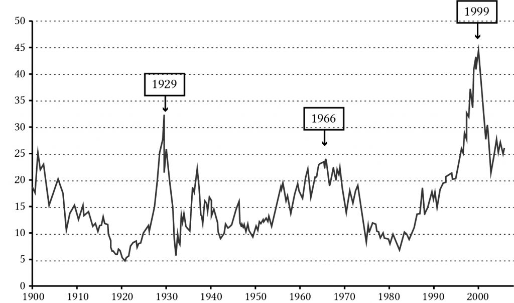
Figure 14.5. Historic PE ratios for UK housing stock.
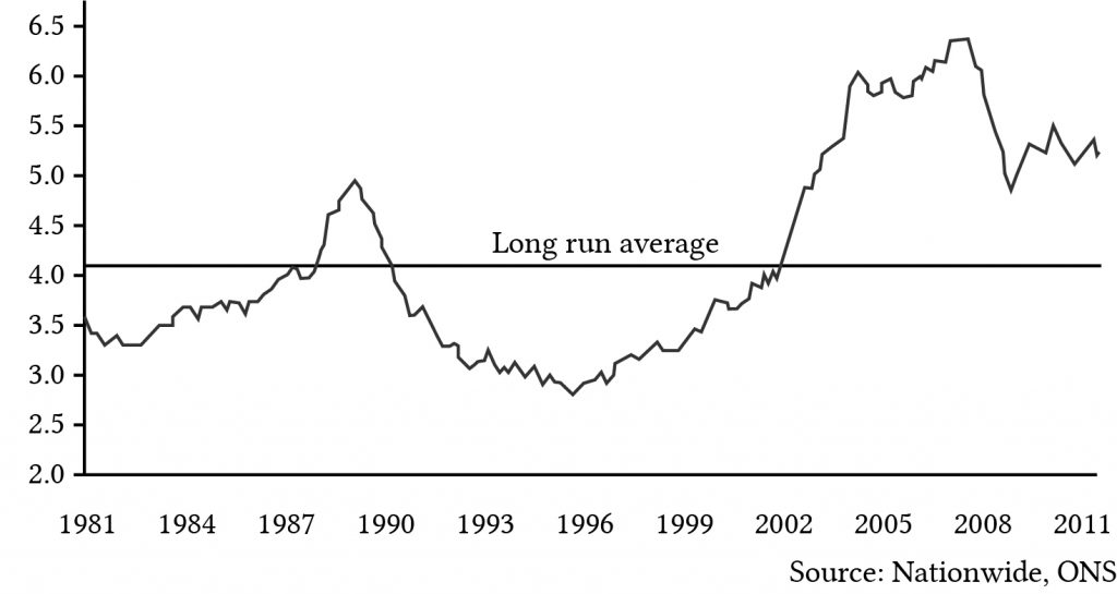
Compare the value of the PE ratios in Figures 14.4 and 14.5. PE values for stocks that reflect depreciable assets (g < 0) have average values around 20. PE values for housing stock that reflect non-depreciable assets (g > 0) have recently averaged around 5. (See Table 14.2.)
Coverage (C) Ratios
Investments can be evaluated according to both profitability and periodic liquidity criteria. Profitability analysis focuses on whether the acceptance of an investment will increase the investor’s present wealth. Periodic liquidity measure analysis considers whether an investment will generate cash flow consistent with the terms of financial capital, especially debt capital, that are used to finance the investment. Is an investment capable of generating sufficient net cash flow in each period to satisfy the requirements for repayment of the loan’s principal plus interest? If not, then the investment is illiquid because liquid funds drawn from other sources are required to meet cash flow requirements associated with the investment. Thus, a simple test of investment liquidity is to compare the net cash flow generated by the investment in a given period with the debt-servicing requirement.
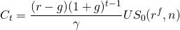
The ratio of net cash flow in a period t, Rt, divided by the loan plus principal payment in the same period, At, is called the coverage ratio, Ct:
(14.17)

If the coverage ratio is equal to or exceeds 1.0,
the investment is liquid in that period. If coverage is less than
one, the investment is illiquid in that period. In most cases, the
loan payment that includes principal plus interest is a constant
“A,” that depends on the price of the purchased asset,
V0; the financed proportion of the purchase
price  ;
the term of the loan n; and the interest rate charged on
the loan rf. Using our previous notation, we
can express the relationship between the amount financed, the fixed
loan payment, the interest rate on the loan, and the term of the
loan as:
;
the term of the loan n; and the interest rate charged on
the loan rf. Using our previous notation, we
can express the relationship between the amount financed, the fixed
loan payment, the interest rate on the loan, and the term of the
loan as:
(14.18)
We solve Equation \ref{14.18} for A and substitute the result for At in Equation \ref{14.19}. In the same equation,we also substitute R0(1 + g)t for Rt, and obtain:
(14.19)
Replacing V0 with [R0 (1 + g)]/(r – g), we can rewrite Equation \ref{14.19} as:
(14.20)
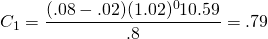
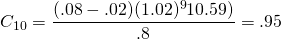
We illustrate Equation \ref{14.20} as follows. Assume r = 8%, g = 2%, n = 20, and rf = 7%. Also assume the investment is 80% financed. Using an Excel spreadsheet, we find that US0(7%, 20) = 10.59.
Table 14.3. Calculating
US0(rf=7%,
n=20)
Open Table 14.3 in Microsoft Excel
| B6 | Function: | =PV(B3,B4,B5,,0) | |
| A | B | C | |
| 1 | Calculating US0(rf = 7%, n=20) | ||
| 2 | |||
| 3 | rate | 7% | |
| 4 | nper | 20 | |
| 5 | payment | -1 | |
| 6 | NPV | $10.59 | “=PV(rate,nper,payment,,0) |
Then we find the coverage value for the first year of the investment to equal:
(14.21a)
Interpreted, in year one, the investment described above will only pay for 79 percent of the loan payment due. However, 10 years later and half way into the term of the loan, the coverage ratio has increased to:
(14.21b)
Finally, in the last year of the loan, the coverage ratio is:
(14.21c)
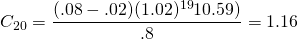
In other words, in year 20, the last year of the loan, the investment cash flow not only repays the loan but 16 percent more than the required loan payment. Of course, after the loan is repaid, the periodic cash flow is available to the firm to meet its cash flow requirements.
One word about the term of the investment, it is assumed to be infinite. However, for any one investor, the term may be finite, but since the terminal value for any one owner is simply the present value of the continued cash flow, we can express the investment as having an infinite life. Therefore, we are justified in ignoring the term of the infinite-life investment.
When is the coverage equal to 100 percent? There is another way to approach the issue of coverage. It is to ask in what year is the coverage equal to 1? To answer this question for the geometric growth model with an infinite life and using the already established notation, we set:
(14.22)
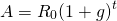
and solving for t we find:
(14.23a )
And after making substitutions for A and R0 and simplifying, we can write:
(14.23b )
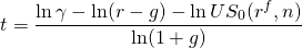
We illustrate equation using numbers from the
previous example where:
= .8, r = .08, g = .02, rr =
.07, and n = 20. We find:
(14.24 )
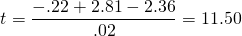
In words, what we have found that the 12th payment will be the first period that more than pays for its financing.
Summary and Conclusions
An investment may earn two types of returns: time dated cash flow and capital gains (losses). Moreover, these returns can be earned over the lifetime of the asset. The relative importance of the two forms of returns, cash flow versus capital gains (losses), will determine the inter temporal liquidity of the asset. The greater the portion of the return is earned as cash, the more liquid will be the investment.
This chapter demonstrated whether an investment earns capital gains (losses) is determined in PV models by its pattern of expected future cash flow. Expected increases (decreases) in the number, frequency, or amount of the expected future cash flow will produce capital gains (losses). Inflation causes long-term investments to become less liquid because they increase the rate of growth in the investment’s cash flow.
Investments that earn capital gains are called appreciating investments. Investments that experience capital losses or depreciation are referred to as depreciating investments.
Perhaps paradoxically, investments that earn capital gains are less liquid than investments that experience capital losses. Assuming investments earn similar total rates of return, the greater the cash returns are compared to total returns, the greater are the liquid funds available to meet liquidity needs including repayment of funds and interest required to maintain control of the asset.
In this chapter we developed current-to-total returns (CTR) measures to indicate an investment’s liquidity over time. Furthermore, CTR measures were shown to be related to price-to-earnings (PE) ratios which also depended on an investment’s liquidity. Finally, one feature of an investment, is its coverage, its ability in any one period to repay principal and interest payments due in any one period. If funds borrowed to purchase an appreciating investment are repaid with a constant loan payment,then initially, it is likely that cash flow generated by the investment will not cover the interest and principal payments. This pattern is very likely during periods of inflation. Coverage ratios will also indicate the liquidity of investments over their productive lives.
In summary, the periodic liquidity of an investment is an important characteristic that should influence the capital decisions of financial managers along with the impact of an investment on the firm’s solvency, profitability, efficiency, and leverage.
Questions
- Please describe three possible appreciating and three depreciating investments that are available for most farm financial managers.
- Describe the connections between capital gains (losses) with an investment’s periodic liquidity.
- Describe the connection between the inflation rate i and an investment’s CTR ratio.
- How is an investment’s periodic liquidity related to its CTR (current-to-total returns) ratio and its C (coverage) ratio? How are the two periodic liquidly measures related to each other?
- Compare the firms current (CT) ratio and its debt-to-service (DS) ratio with an investment’s CTR ratio and C ratio. In what ways are they similar? How do they differ?
- Consider the CTR ratio described in Equation \ref{14.3}. Find the CTR ratio for the investment whose anticipated cash flow is a constant R in perpetuity described below:
(Q14.1)
(Hint: Observe the CTR ratio described in Equation \ref{14.3}. Then derive capital gains (losses) measures for the PV model described in this question.)
- Find the CTR ratio for an investment whose defender’s IRR is 8% and its anticipated growth rate is 2%. Then find the PE ratio for the same investment.
- Assume that PE ratios can be approximated using Equation \ref{14.10}. What would account for the large swings in PE ratios described in housing stock described in Figure 14.2—changes in expected r or g? Or due to some other influence on the value of housing stock?
- Find the coverage (C) ratio for year 5 for the investment
described in the text where:
= .7, r = .08, g = .02, rr =
.07, and n = 20. Call the result, the result for the base
model.
- Recalculate the base model C ratio where n = 20 is changed to n = 15. Describe how reducing n changed the coverage compared to the base model. Then provide an explanation for the change in coverage.
- Recalculate the base model C ratio where g = .02 is changed to g = –.02. Describe how reducing g changed the coverage compared to the base model. Then provide an explanation for the change in coverage.
- Recalculate the base model C ratio when
= .8 is changed to
= .6. Describe how increasing γ changed the coverage compared to
the base model. Then provide an explanation for the change in
coverage.
- In this chapter we derived Equation \ref{14.18} which solved
for the time period in which the coverage was 100%. Find the time
period in which coverage is 100% when
= .7, r = .08, g = .02, rf =
.06, and n = 20. Call the result, the base model result.
Then use Equation \ref{14.18} to find how t associated
with 100 percent coverage changes for the following cases:
- Recalculate the base model and find a new t value associated with 100% coverage where n = 20 is changed to n = 15. Describe how reducing n changed t and then provide an explanation for the change in t.
- Recalculate the base model and find a new t value associated with 100% coverage where rf = .06 is changed to rf = .08. Describe how increasing the interest rate rf changed t associated with 100% coverage. Then provide an explanation for the change in t.
- Recalculate the base model and find a new t value associated with 100% coverage where r = .08 is changed to r = .06. Describe how decreasing the discount rate r changed t associated with 100% coverage. Then provide an explanation for the change in t.
- Suppose the firm you managed was facing financial stress due to falling prices. Moreover, the stress is reflected in low liquidity and solvency measures for the firm. It appears that there is no way the firm can survive its current crises without liquidating not only short-term assets, but also long-term investments. Based on what you have learned about investment liquidity, propose a plan for the firm to meet it liquidity crisis.