
13: Homogeneous Investment Types
- Page ID
- 12758

After completing this chapter, you should be able to: (1) distinguish between incremental and stand-alone investments; (2) understand how time and use costs determine the optimal service extraction rate from investments; (3) distinguish between net present values (NPV), annuity equivalent (AE), and internal rates of return (IRR) used to measure earnings by an investment or by equity committed to funding an investment; and (4) use Excel spreadsheets to find NPV, AE, and IRR for investments and equity funds committed to some practical multi-period investments.
To achieve your learning goals, you should complete the following objectives:
- Learn how to distinguish between incremental and stand-alone investments.
- Learn how an investment’s time and use costs determine its optimal service extraction rates.
- Learn how an investment’s liquidation and acquisition values determine its fixity.
- Learn how to find contributions from incremental investments by finding changes in the firm’s cash receipts (CR), cash cost of goods sold (COGS), cash overhead expenses (OE), and change in operating and capital asset accounts.
- Learn how the order of changes influences the returns on incremental investments.
- Learn how to project cash flow and changes in operating and capital accounts.
- Learn how to use Excel templates to find NPV, AE, and IRR measures earned by investments or by equity committed to some practical multi-period investments.
Introduction
The nature of investments. An investment is a commitment of resources for one or more periods. We invest instead of consume because we expect future investment earnings will more than compensate for the present investment sacrifice. If the commitment is to a firm, we talk about return on the firm’s assets (ROA). If the commitment is to an investment, we talk about the returns on an investment (ROI). However, since it is more common to use PV models to examine returns on an investment rather than a firm, rather than differentiate between commitments to a firm or an investment, we will refer to both as investment analysis. To make things a little more confusing, rather than introduce a new acronym, ROI, that would undoubted annoy the amazing editor of this book, we will refer to both returns on an investment and returns on the assets of a firm as ROA measures.
Returns on an investment versus returns on equity invested in an investment. We are interested in the rate of return on funds committed to an investment. We are also interested in the rate of return on equity committed to an investment. The main distinction between measures that reflect earnings on an investments and equity funds committed to an investment is the following. Returns on equity subtract from total returns interest costs earned by debt capital. Returns earned by the investment do not subtract interest costs earned by debt capital.
Return measures. In previous chapters and especially in the previous chapter we described several measures designed to measure the returns earned by an investment versus returns earned by equity committed to an investment. These measures include NPV that find the present value of profit earned by the investment or equity committed to the investment over its economic life. AE derived from NPV convert the present value of earnings to their equivalent annuity—the constant amount that could be paid each period over the economic life of the investment. Finally, IRR measure the average rate of return earned by the investment or by equity committed to the investment earned over its economic life.
Two kinds of investments. There are two kinds of investments: stand-alone and incremental. Stand-alone investments are independent of other investments. They are self-contained. Furthermore, we do not expect that increases or decreased in stand-alone investments will influence the returns or affect investment decisions of other investments. Stand-alone investment may include more than one capital investment but when they do—they are interdependent so that one investment cannot be studied independent of the other investments.
Incremental investments add to, replace, or modify existing investments. Therefore, when considering the PV of incremental investments, we must account for the contributions of other inputs and services from other investments. In most studies, we ignore the problem of incremental investments by assuming that we can measure their contributions independent of the contributions of other investments and nondurable inputs—treating them as stand-alone investments. The reality is quite different. Most of our investments are incremental ones and measuring their unique contributions is difficult because when we add an investment to another investment(s), the use of other investments and nondurable inputs often change as well—making it difficult to identify what part of the change in the investment’s returns and expenses we can attribute to the new investment.
Investment identities. Capital investments have a distinct property. They can supply services for more than one period without losing their identity and without exhausting their service potential. Think of a battery as an example. It can provide services for more than one period without losing its identity. Another property of capital investments is that their service extraction most often requires services from other durables and nondurable inputs–whose service capacity and identity change with a single use.
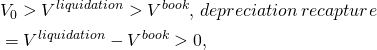
Fixed investments. A fixed investment is one already owned by the firm and unlikely to be removed from service. Glenn Johnson describe the conditions required for an investment to be fixed; namely, that the investment’s acquisition value (V0) and liquidation value (V0liquidation) bound its value in use (V0use). In other words an investment is fixed or unlikely to be removed from service if: V0liquidation < V0use < V0. Because the investment’s value in use is less than what it would cost to acquire another one and because its liquidation value is less than what it is earning—the firm has no incentive to invest or disinvest in them. An investment with a zero or negative liquidation value is one likely fixed as long as it contributes something positive to the firm.
Accrual income statements (AIS) and investment analysis. An AIS makes no effort to find the contributions of a single or subset of a firm’s investments. However, isolating earnings from a single or subset of the firm’s investments is exactly what we do when constructing PV models for incremental capital investments—we attempt to isolate returns from capital investments that add to, replace, or alter capital investments used by the firm. Otherwise, we have no basis for incremental investment decisions.
ROA, ROE, and IRR. AIS summarize the collective contributions of a firm’s assets and equity during a single period by accounting for cash flow and changes in operating and capital accounts. Furthermore, we can calculate AIS earning measures as a percentage of the firm’s beginning assets and equity and report them as one period ROA and ROE respectively. Incremental investment analysis finds IRR for investments and equity committed to investments for one or several periods and report the results as the internal rate of return earned by an investment (IRRA) and internal rate or return earned by equity committed to the investment (IRRE). To find IRRA and IRRE for incremental investments require that we find the incremental investment’s unique contributions over their economic life. As a result, we cannot use the firm’s AIS to evaluate an incremental investment, although we organize our analysis around changes in operating cash flow and changes in operating and capital accounts—just the same as we did when analyzing a firm or stand-alone investment.
What follows. To find NPV, AE, IRR that reflect investment earnings and equity committed to stand-alone and incremental investments, we organize the remainder of this chapter as follows. First, we describe the connection between incremental and stand-alone investments. Second, we describe how to project cash flow and changes in operating and capital account used to describe stand-alone and incremental investments. We are careful when calculating NPV, AE, and IRR to indicate returns on stand-alone versus incremental investments whether they measure returns on the investment or returns from equity committed to the investment. Finally, we demonstrate how to find NPV, AE, and IRR for several practical multi-period stand-alone and incremental investments problems using Excel spreadsheets.
Incremental Investments
Incremental investment analysis intends to separate the contributions of an incremental investment from those of existing investments and other nondurable inputs and services. To be clear, incremental investment analysis does not hold all other inputs constant when considering its contributions because doing so would underestimate its contributions and lead to less than optimal investment choices.
The contributions of a stand-alone versus an incremental investment. To emphasize the connection between a stand-alone and an incremental investment, consider investing in scissor-type investments whose blades we purchase separately. With only one blade, the scissors’ output is small—equivalent to a knife. When we purchase a second blade, the scissor output increases toward normal. However, the increase in the scissors’ production when we added the second blade changed because we changed the use of both blades. If we analyzed the contribution of the second blade keeping the first blade idle, output would have remained low. Is it fair to attribute to the second blade the contributions of the first blade? Yes, and that is the approach we follow in incremental investment analysis because we want to know how adding the second blade changes the productivity of the scissors. Since the firm already owns the first blade, the investment decision focus is on the second blade, not the first one.
Optimal Service Extraction Rates
We want to determine the rate of return on multi-period capital investments. In this analysis, we assume that our investment provides services at its optimal rate. Finding the optimal service extraction rate for capital investments is complicated and we often employ complex computer programs to find these optimal rates. To do so, we must determine the optimal rate at which to extract services from our capital investments. At our level of investment analysis, we assume that optimal service extraction rates have already been determined. Yet it is important to understand what determines optimal service extraction rates even though the focus of our analysis is on the investment’s rate of return.
To be clear, when we discuss the cost of extracting services from our capital investment, we include its change in salvage value, the cost of using other nondurable inputs, and the change in the value of other capital investments whose services support our investment. As it turns out, the costs of using a capital investment within a period conform to the categories already identified in our PV templates. The cost of using nondurable inputs are measures as cash costs of goods sold (COGS). The cost of extracting capital investment services that depend mostly on the passage of time, we measure as cash overhead expenses (OE). The cost equal to the change in the liquidation value of the capital investment we measure as depreciation (Dep) and most of the time we assume that this rate of depreciation is determined by the passage of time.
Service extraction rates when the cost of using the investment depends mostly on the passage of time. Consider, for example, an investment whose use cost depends mostly on the passage of time such as a storage facility. The roof, for example, has a finite time during which it can provide services. It simply wears out over time. Much the same is true for other parts of the building including its painted surfaces, floors, and other building features. While there may be some important costs associated with heating, ventilation, and air conditioning services, these costs depend mostly on the passage of time and weather conditions than on the amount of items stored or the activity that occurs in the building. Finally, investments in buildings are usually fixed because their liquidation value is often low. To use a building requires that the new owner relocate to the building site. Thus, location fixity reduces the liquidity of the investment and contributes to its fixity in the firm’s investment portfolio.
So what is the optimal use of an investment whose costs depend mostly on the passage of time and whose low salvage value contributes to its fixity within the firm? Since its marginal use cost is usually low, their optimal use is their maximum capacity as long as the investment is making some positive contributions to the firm. For investments whose use costs depend mostly on the passage of time, we are not likely to change their use when adding an incremental investment to the firm unless we operate them at less than full capacity before the incremental investment.
Service extraction rates when the cost of using an investment depends mostly on its use. Consider another kind of investment whose use costs depends mostly on services provided by other capital investments, including maintenance costs, and nondurable inputs. Electric motors or gasoline powered equipment have their cost of service extraction dependent mostly on the cost of using nondurable inputs and services from other durables.
So what determines the optimal service extraction rates from investments whose cost depends mostly on use and other inputs? The optimal service extraction rate depends mostly on the marginal use costs. Furthermore, we expect that service extraction rates change when incremental investments are added to the firm that alter these marginal use costs. In sum, investments whose costs depends mostly on their use will find that their optimal use is not fixed nor at their maximum capacity.
Opportunity costs. All investments that provide services for one period or more incur opportunity costs equal to the defender’s IRR times the value of the investment at the beginning of the period. We incur the cost when we sacrifice a defending investment to employ a challenging one. We account for these costs when discounting future costs and returns to their present value.
Therefore, when we analyze incremental investments that provide services for more than one period, we must account for their opportunity cost and treat them as a mostly time related cost and unlikely to influence optimal service extraction rates within the period.
Least cost expansion paths. We have described how the optimal service extraction rates for stand-alone and incremental investments depend on whether the cost of extracting services depend mostly on their use or the passage of time. If the cost of extracting services depends mostly on the passage of time, their use will not likely change even with the addition of an incremental investment.
On the other hand, if the cost of extracting services from an investment depends mostly on its use, then their optimal service extraction rates will depend on the variable cost of using other inputs and the marginal use cost of extracting services from other investments.
To find the optimal service extraction rate, we employ a tool from economic analysis we refer to as the least-cost expansion path that we describe in Figure 13.1.
Figure 13.1. A least cost expansion path that employ other inputs (OI) and capital investment services (CS) to produce outputs Q1 and Q2 using various combinations of OI and CS.
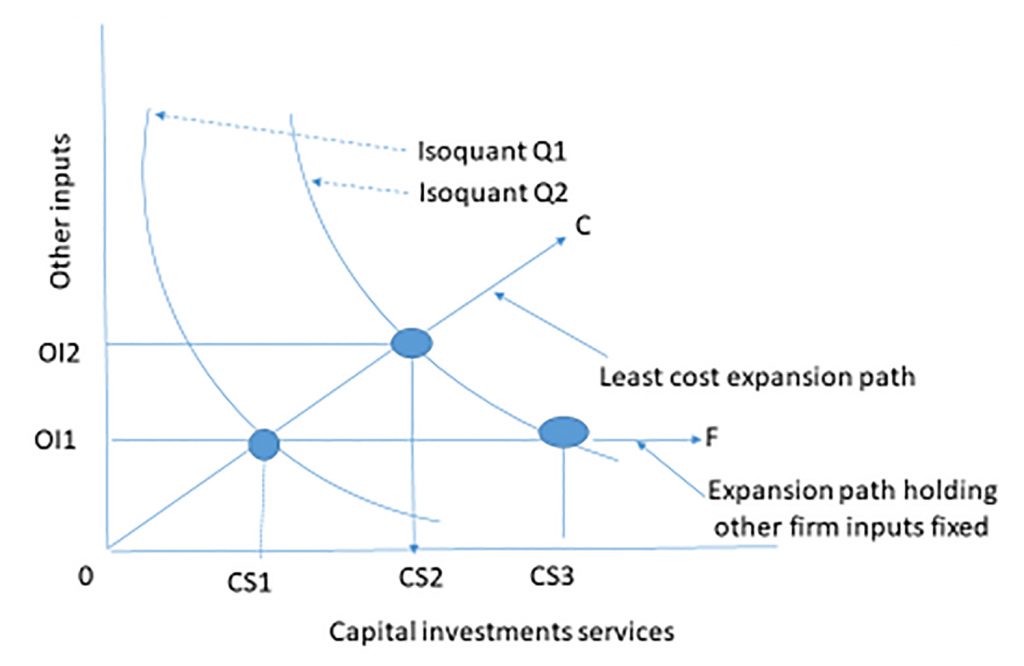
Assume that a firm produces output using a combination of capital services and other inputs. We graph the combinations of capital services and other inputs that produce the same output and call the result an isoquant (i.e. same quantity). In Figure 13.1 we represent two levels of output by isoquants Q1, and Q2 drawn convex to the origin to reflect diminishing marginal productivity—a subject covered in microeconomics.
Now suppose that the firm considers a capital investment that will allow the firm to increase its use of capital services from CS1 to CS3 and increase output from Q1 to Q2. If the cost of using other inputs depend mostly on the passage of time, we hold their contributions fixed at OI1. On the other hand, if the cost of using other inputs is variable, then economic production theory teaches that increasing production from Q1 to Q2 holding other inputs constant would be inefficient. Instead, the theory teaches that the firm should increase capital services and other inputs along some least cost line OC determined by the relative costs of increasing both the capital services from the new investment and from the other inputs.
Increasing production along the least cost line OC, the firm would increase capital service from CS1 to CS2 an amount less that was required to reach Q2 when we held other inputs constant. In other words, increasing the use of other inputs allowed the firm to use less capital services from the new investment compared to the capital services required if other inputs were held constant (CS2 – CS1) < (CS3 – CS1) while still producing the same level of output. Furthermore, expanding other inputs and services from the new durable along the least cost expansion path assures us that the cost of increasing other inputs from OI1 to OI2 is more than offset by reducing the cost of capital services from (CS3 – CS1) to (CS2 – CS1).
Which expansion path? We have demonstrated that whether to measure the cost of increasing production along the least cost line OC or the expansion path OF that holds other inputs constant at OI1 depends on the nature of the costs of increasing the use of other inputs depends mostly on the passage of time or use. If increases in other inputs makes the investment more productive, this productivity increase is credited to the investment. Finally, if we measure changes along the least cost path, we must recognize that we are answering a different kind of question than “what are the unique returns to a challenging investment?” When performing PV analysis on a stand-alone investment, we ask: does the investment earn a positive net present value (NPV)—greater than the PV sacrificed by liquidating the defender. In contrast, the incremental investment analysis asks: is this change in the capital structure of the firm and use of other inputs more efficient and profitable than before the change?
Incremental investments and comparing two challengers. Incremental investment analysis is a legitimate approach for attempting to isolate the change in a firm’s revenue and cost in response to an incremental capital investment and changes in the use of other inputs. We justify the incremental approach because we are adding an incremental investment that may change the optimal use of other nondurable inputs and use of existing durables.
But what about a firm choosing between two or more challenging investments? In this case, three scenarios are being considered: the defending firm with its existing capital structure and the firm with incremental investments one and two. In some instances, the analysis finds the present value difference between the two incremental investment’s cash flow discounted by the defender’s IRR. Although this approach is convenient, it not generally an acceptable approach.
The problem of discounting the cash flow difference between two possible incremental investments is that we design NPV models to rank only two investments, not three. We illustrate the problem of ranking two challengers using their differences and the defender’s IRR as the discount rate. In our example, we assume the defender’s IRR is 12% and incremental challenging investments C1 and C2 have similar two-period terms with the following cash flow:
Table 13.1. Ranking
investments C1, C2,
and the difference (C1–C2) with
rankings in parentheses
| Period | Cash flow for C1 | Cash flow for C2 | Cash flow for (C1–C2) |
| 0 | –$10 | $15 | –$25 |
| 1 | $1 | 1 | 0 |
| 2 | $15 | -$10 | $25 |
| NPV at 12% |
$2.85 (2) |
$7.92 (1) |
–$5.07 C2 is preferred to C1 |
| IRR |
27.58% (1) |
–21.62% (2) |
0% Indifferent between C1 and C2 |
The first thing to note about the example is that NPV(C1) minus NPV(C2) equals NPV(C1–C2) Therefore, individual NPV rankings in this example are consistent with NPV difference rankings as long as their cash flows are independent. However, IRR and NPV rankings for C1 and C2 are inconsistent because they violate size homogeneity conditions. Furthermore, IRR rankings depend on multiplicative operations. As a result, IRR rankings for C1 versus C2 are inconsistent with the IRR of C1 versus C2 based on the IRR of the difference in cash flows (C1–C2).
Forecasting Future Values for PV Templates
Future values for PV template variables. Chapter 12 introduced two PV templates, one for assets and one for equity. We illustrated the templates in Tables 12.5 through 12.7 using period one data reported in the coordinated financial statements (CFS) for HQN. The two templates apply regardless of whether we are analyzing the PV of incremental or stand-alone investments. We now ask, where can we find future values for template variables that will permit us to solve multi-period PV incremental or stand-alone problems? The answer is that we estimate (guess) their values!
Excel PV templates often create a tab for each exogenous variable as well as a tab for discount rate and tax rate assumptions. These tabs feed exogenous variable values to the PV templates that calculate NPV, AE, and IRR. The columns/tabs may include:
- Investment. Typically, there will be several investment components for a project aggregated to a single value for the PV tab. In addition, some investments may take place over the course of the project. For example, for long-term projects, earnings may be reinvestment in shorter-lived investments. In the case of dairy expansions populated with purchased cows, there will be an initial investment followed by reinvestments of cows until the herd can generate its replacements.
- Annual investment market liquidation values.
- Annual investment accounting book value. This tab must also include depreciation schedules.
- Annual account balances.
- Annual CR that may reflect a wide range of patterns over the investment’s economic life including no change, constant rate of change, lower receipts in start-up years, growth to a plateau followed by a decline, and several years with no receipts followed by growth to a plateau followed by a decline (e.g., orchards).
- Annual cash COGS.
- Annual cash OE.
Our confidence in the estimates of future values for exogenous variables decreases as the distance in time of the projection from the present increases—simply because we know more about the present than the future. Still, our estimates of near present exogenous variable values are often seriously wrong. For example, present investment amount is usually a well-documented number. Nevertheless, we frequently hear reports of investment expenditure overruns. Yet current and recent past data may still represent our best starting point for projecting future exogenous variable values.
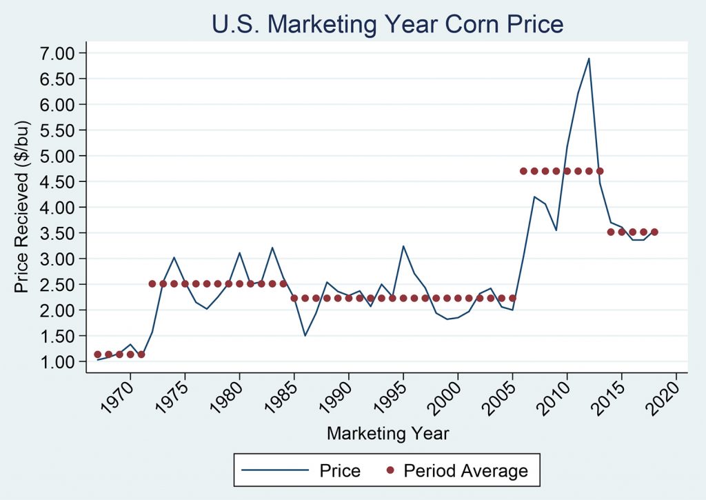
We often project future values as stable trends. However, the future is hardly ever so predictable. Consider, for example, nominal corn prices in the mid-1960s. Corn rice fell by two and one-half times in the 1970s, leading to a fall in related prices and the financial crisis of the 1980s. Land values fell as much as 50 percent. Later, in the 2006–2013 period corn prices nearly doubled over the previous twenty-year period only to fall again in 2013 with input prices substantially higher than in the previous period. In real terms, current profitability is lower than in was in the post 1980’s period.
Historically, it has taken grain and oilseed markets six to twelve years to find their “new normal” following large, sustained shocks. History again provides a guide to the future, but the internal confidence around these future projections should be wide.
There are research groups such as the Food and Agricultural Policy Research Institute (FAPRI) at the University of Missouri (fapri.missouri.edu/publication/2019-u-s-baseline-outlook/ FAPRI) who annually make 10-year baseline projections for grain, oilseed, livestock markets, and a variety of other indicators. Even here, it is important to moderate forecasts using microeconomic principles and experience in making projections including a range of scenarios. Understanding intermediate and longer-term industry supply curves including regional and international dimensions is very important for most projects.
Figure 13.2. Past, Current, and Forecasted values for Corn Prices in the U.S. from 1965 to 2020 (National Agricultural Statistics Service).
Testing for robustness. That we populate our PV templates with estimates suggests that our templates will not be completely accurate. They will be consistent because the templates relate variables to each other consistently, but they are not likely to be completely accurate. We simply are not likely to estimate all of the future values of our variables correctly. As a result, we should calculate NPV, AE, and IRR under a variety of assumptions about future values so that we have some impression about the robustness of our estimates.
Exogenous and Endogenous variables in the PV templates. Similar to CFS, we populate PV templates with exogenous and endogenous variables. The distinction we made between exogenous and endogenous variables when constructing CFS is modified only slightly when constructing PV templates. The distinction is required because CFS modeled financial activity for one period. PV templates can model financial activity for several periods, requiring that we project variable values for future periods.
We define exogenous variables in PV templates as those whose values are determined outside of the template. We define endogenous variables in PV templates as those whose values are determine by current and previous values of template variables.
We can identify exogenous variables within the template because their cell values do not reference variable values in other cells. We can identify endogenous variables within the template because they include a formula signaled by an “=” sign that references other cells.
We must project all variables values in a PV template except some of those described at the beginning and end of period one. What distinguishes between projected values is whether we project their values using current and previous periods or whether they are projected outside of the PV template. Projections made using current or previous period template values are endogenous. Projections made outside of the PV template are exogenous.
Expert opinion and forecasts. Often, we rely on experts to project revenue related variables such as yields, prices, sales, and margins between revenue and cost. For example, services such as the Food and Agricultural Policy Research Institute (FAPRI) at the University of Missouri (fapri.missouri.edu/publication/2019-u-s-baseline-outlook/ FAPRI) presents a summary of 10-year baseline projections for U.S. agricultural markets, farm program spending, farm income and a variety of other indicators. Extension specialists, such as Dr. Jim Hilker, who have distinguished themselves with accurate forecasts can also be an invaluable resource.
Populating the PV Templates
We now describe in more detail the variables and data needed to populate our PV templates that enable us to find rolling NPV, AE, and IRR estimates for investments and invested equity. We begin with the only information we know for sure, future dates: 2019, 2020, 2021, etc. Therefore, we begin populating our PV models templates with the one thing we know about the future: future dates recorded in column 1.
The investment acquisition amount. In both the investment and equity PV templates, we record the investment acquisition amount in cell B4. Its value is determined outside of the template making it an exogenous variable. We treat the investment’s acquisition value as though it were a cash expenditure unless funded by debt, an amount recorded in cell C4. When we employ debt to acquire the investment, the focus is on the equity invested—equal to the investment amount less the debt used to acquire the investment. The investment amount may be the most accurate data in our template because investments occur mostly in the present and we know much more about “now” than “later”.
The investment amount is usually a well-documented number. Durable sellers post their offer prices. Markets establish and record durable exchange prices. References for used farm equipment similar to Kelly’s Blue Book for cars are generally available.
Complicating our investment data are projects that incur investments costs over several time-periods. Indeed, one might consider repair and maintenance expenditures designed to improve the life and durable performance to represent additional investments. In other cases, the investment includes several durable that we replace at different intervals. For example, feeder calf operations routinely replaces one cohort of calves with another but the feeding equipment and physical facilities we replace less often than the feed calves.
Liquidation values. To find rolling NPV, AE, and IRR estimates, we require not only an investment acquisition amount, but investment liquidation and market values over time. An investment’s acquisition value, V0, is the amount of money exchanged to acquire the investment. An investment’s book value, Vbook, equals it acquisition value minus its accumulated depreciation. An investment’s liquidation value, Vliquidation, is the amount of money a buyer is willing to exchange for the investment when it the investment is sold. If an investment’s liquidation value is greater than its acquisition value, we refer to the difference as capital gains. If an investment’s liquidation value is less that its acquisition value but greater than its book value, we refer to the difference as depreciation recovery. Finally, if the liquidation value is less than its book value, we refer to the difference as capital losses. We describe capital gains, depreciation recovery, and capital losses in the following equations:
for
(13.1)
 V_0 > V^{book}, \,capital\, gains\, = V^{liquidation} - V^{book}
> 0, \end{equation*} " title="Rendered by
QuickLaTeX.com">
V_0 > V^{book}, \,capital\, gains\, = V^{liquidation} - V^{book}
> 0, \end{equation*} " title="Rendered by
QuickLaTeX.com">
for
(13.2)
 V^{liquidation} > V^{book}, \,depreciation\, recapture\, \\
& = V^{liquidation}- V^{book} > 0, \end {split}
\end{equation*} " title="Rendered by QuickLaTeX.com">
V^{liquidation} > V^{book}, \,depreciation\, recapture\, \\
& = V^{liquidation}- V^{book} > 0, \end {split}
\end{equation*} " title="Rendered by QuickLaTeX.com">
and for
(13.3)
 V^{book}> V^{liquidation}, \,capital\, losses\, = V^{book}-
V^{liquidation} > 0. \end{equation*} " title="Rendered by
QuickLaTeX.com">
V^{book}> V^{liquidation}, \,capital\, losses\, = V^{book}-
V^{liquidation} > 0. \end{equation*} " title="Rendered by
QuickLaTeX.com">
We determine accounting book values by applying tax regulations that specify depreciation amounts depending on the type and age of the investment. Since depreciation forecasts depend on the age and amount of the investment, we generally consider them endogenous variables. Furthermore, we recognize that liquidation values of investments are also generally determined by projecting market values and cost data and may be endogenously or exogenously variables. When we do not expect to liquidate the investments, but want to estimate their NPV, AE and IRR, we may equate market liquidation value with book values.
Endogenous variables in PV templates. When projecting COGS data we generally assume they are related to CR projections. COGS are likely to depend on CR because they mostly vary with production levels making them endogenous variables. However, COGS may also vary with time as relative supplies of inputs and inflation add a trend line to our COGS estimates. We might express this relationship between future value of COGS, an endogenous projection, and their connection to CR and time t as:
(13.4)

where  and
and  are estimated in such a way to reduce the average error in period
t, εt, involved in the estimation of
COGS while treating time t and CR as exogenous variables.
When we have past values of the variables in Equation \ref{13.4} we
can use statistical techniques such as linear regression analysis
to find the coefficients.
are estimated in such a way to reduce the average error in period
t, εt, involved in the estimation of
COGS while treating time t and CR as exogenous variables.
When we have past values of the variables in Equation \ref{13.4} we
can use statistical techniques such as linear regression analysis
to find the coefficients.
Similarly, we can treat future OE as endogenous and estimate then from values of other variables. However, OE in contrast to COGS we expect to be more related to time and their previous values than CR values. This connection between OE, time and their previous values we can express as:
(13.5)

where  are estimated in such a way to reduce the average error in period
t, εt.
are estimated in such a way to reduce the average error in period
t, εt.
Endogenous variable projections. We often begin building a PV template data set by observing previous values of exogenous and endogenous variable reported in the current and past CFS. For example, suppose that we observe that prices and yields in the past have predictable trends and changes. We might use these observations of past template variable values to project their future value. To illustrate, suppose that over the past 10 years, corn yields g1, g2, ⋯, g10 have increased by 13%. Then letting [/latex]\bar{g}_y[/latex] equal the average percentage increase in corn yields we find its value in the equation equal to:
(13.6)

And solving for the annual average increase in yield we find:
(13.7)
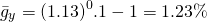
Assuming the past trends in yield continue and if the yield last year were 140 bushels per acre, in 5 years we would expect yields to have increased to:
(13.8)

Finally, assume we employ the professional forecasting services to find future values corn prices which when multiplied by our projected yields produces an estimate of CR.
Projecting margins. One of the main ways we can improve our variable value forecasts is to observe their values and relationships to one another in the past—and the more observations, usually the better. One observation that is important using past data is the margin between revenue and costs. We can be confident that this difference is bounded, otherwise, competitors would flock to join our industry and begin replicating our operations. If the difference is negative for a significant period of time, we will become insolvent and leave the industry.
Past margin observations may guide our projection in the future. Taxes will be some function of the difference between revenue and sales. Changes in comparatives advantages and preferences may also be included in the description of how the variables are related. Future preferences will influence demand for what we produce. Changes in comparative advantage—who can produce least expensively and where—will also influence revenue and expenses. Favorable increases in comparative advantage will reduce our costs and put us in a position to expand our operation. And as we increase in sophistication, we might worry about local, national, and international politics that may influence tariffs and the challenges of competing in a global economy.
Other forecasts. Sometimes, failing to find forecasts of direct interest to the calculation of our investment’s NPV, AE, and IRR—we can often times find forecasts highly correlated with our forecasts of interest. For example, suppose we are interested in the price of hard red winter wheat but can only observe past prices of corn and soybeans. Using linear regression, a statistical technique that allows us to relate an endogenous variable to one or more exogenous variable—we can use the future estimates of corn and soybean prices to predict hard red winter prices.
Real versus nominal data values. In our PV templates, we project CR, cash COGS and cash OE. We can employ several assumptions about future cash flow associated with these values. The first one is that there is no change from data entered in year one. This assumption is consistent with capitalization formula that assume zero change in future cash flow. It may also be relevant if the model assumes that data are in real numbers so that numbers do not change with inflation. Furthermore, we may assume that the future is represented by the present and these relationships between variables in the present should be preserved.
Solving Practical Investment Problems: Green and Clean Services
Lon is considering investing in a lawn care and snow removal business that will require that he purchase lawnmowers, snow blowers, and other equipment. Lon intends to name his business Green and Clean Services (GCS). Assume that Lon has hired you to advise him on whether or not he should invest in the business. To solve Lon’s investment problem you intend to solve Equation \ref{13.6} (see Equation \ref{12.21} in Chapter 12).
(13.9)
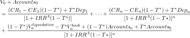
To complete the PV template corresponding to Equation \ref{13.9} and described in Table 12.5, he provides the information that follows.
Acquisition cash flow. Lon estimates the initial investment will cost $40,000. The equipment falls into the MACRS 3-year depreciation class (25%, 37.5%, 25%, and 12.50%) and in four years Lon estimates he can sell his equipment for $10,000. With this information, Lon completes the acquisition stage of his investment analysis.
Operating cash flow. Lon intends to charge $40 per service for both lawn care and snow removal services. He estimates that his expenses (labor, fuel, maintenance) will average $18 per service. Lon projects the number of services for the next four years to be 500 in year one, 750 in year two, 900 in year three, and 1,000 in year four. Lon recognizes that not all his customers will pay for his services when he provides them. He expects his accounts receivable (AR) to equal $1,000 at the end of his first year of operation, to grow to $1200 at the end of year two, to decline to $800 at the end of year three, and to decline to $400 at the end of year four. The outstanding $400 balance at the end of year four, he expects to liquidate when he sells his business.
To simplify, we assume that Lon’s marginal tax rate and capital gains tax rate both equal 20%. Lon also assumes that the before-tax IRR of the defending investment equals 10% and that the after-tax IRR of the defending investment is 8%.
To determine Lon’s operating ATCF, we need to find CR, cash COGS, and cash OE. We begin with CR. CR equals sales less increases (plus decreases) in AR. Increases in AR represent sales for which Lon did not receive payment. Decreases in AR represent previous sales paid for in the current period in cash. We could also adjust CR for increases (decreases) in inventories. But in this example, GCS has no inventories.
To find sales we multiply the number of services per year by the price paid per service. We find that cash sales equal $40 x 500 = $20,000 in year one; $40 x 750 = $30,000 in year two; $40 x 900 = $36,000 in year three; and $40 x 1000 = $40,000 in year four. In year one AR increased by $1,000. As a result, CR equal sales of $20,000 less $1,000 increase in AR or $19,000. In year two AR increased by $200 so that CR equal sales of $30,000 less $200 increase in AR or $29,800. In year three, AR declined by $400 so the CR was greater than sales of $36,000 by $400: $36,000 + $400 equals $36,400. Finally, at the end of year four, the last year Lon intends to operate GCS, AR declines to $400 increasing CR by $400 to $4,400. Finally, the remaining $400 balance of CR Lon liquidates when he sells the business.
Similarly, we find COGS by multiplying the number of services provided times the cost to deliver a service unit. We find they equal $18 x 500 = $9,000 in year one; $18 x 750 = $13,500 in year two; $18 x 900 = $16,200 in year three, and $40 x 1000 = $18,000 in year four.
We calculate depreciation by multiplying MACR 3-year class rates (25%, 37.5%, 25% and 12.5%) times the value of the capital accounts equal to $40,000. Depreciation is ($40,000 x 25%) = $10,000 in year one; $40,000 x 37.5% = $15,000 in year two, $40,000 x 25% = $10,000 in year three, and $40,000 x 12.5% = $5,000 in year four. Finally, we summarize our data and estimations in columns A through M in Table 13.2 below.
Table 13.2. PV Template for
Rolling Estimates of NPV, AE, and IRR for Green
and Clean Services (GCS)
Open Table 13.2 in Microsoft Excel
| A | B | C | D | E | F | G | H | I | J | K | L | M | N | O | P | |
| 3 | Yr | Capital accounts values | Capital accounts liquidation value | Capital accounts book value | Operating accounts values (AR- INV – AP – AL) | Capital Accounts Depr. | Cash Receipts (CR) | Cash Cost of Goods Sold (COGS) | Cash Overhead Expenses (OE) | Tax savings from depr. (TxDepr) | After-tax cash flow (ATCF) from operations | ATCF from liquidating Capital and operating accounts | ATCF from operations and liquidations | Rolling NPV | Rolling AE | Rolling IRR |
| 4 | 0 | $40,000 | $40,000 | $0 | $40,000 | $40,000 | ||||||||||
| 5 | 1 | $0 | $30,000 | $30,000 | $1,000 | $10,000 | $19,000 | $9,000 | $0 | $2,000 | $10,000 | $30,800 | $40,800 | ($2,222.22) | ($2,222.22) | 0.00% |
| 6 | 2 | $0 | $20,000 | $15,000 | $1,200 | $15,000 | $29,800 | $13,500 | $0 | $3,000 | $16,040 | $19,960 | $36,000 | $123.46 | $61.73 | 0.00% |
| 7 | 3 | $0 | $15,000 | $5,000 | $800 | $10,000 | $36,400 | $16,200 | $0 | $2,000 | $18,160 | $13,640 | $31,800 | $8,254.84 | $2,751.61 | 0.00% |
| 8 | 4 | $0 | $10,000 | $0 | $400 | $5,000 | $40,400 | $18,000 | $0 | $1,000 | $18,920 | $8,320 | $27,240 | $17,449.18 | $4,362.30 | 0.00% |
To find after-tax cash flow (ATCF) from operations during each year, we subtract from CR in column G, cash COGS in column H and cash OE in column I and multiply the result by (1 – T*) where T* equals the average tax rate paid on investment earnings that we set equal to 20%. Finally, we add tax savings from depreciation T*Dep reported in column J. These operations on exogenous variables estimate ATCF from operations reported in column K.
Liquidation. At the end of four years of
operating GCS, Lon’s equipment has a salvage value of $10,000 and
an accounting book value of $0. Therefore, the after-tax liquidated
equipment salvage value equals V4 (1 –
T*) = $10,00(1 – .2) = $8,000. (See equation
13.6). The AR account has a value of $400 and when liquidated is
treated as after-tax cash income of AR4(1 –
T*) = $400(1 – .2) = $320. The sum of ATCF from
liquidation is equal to $8000 + $320 plus 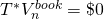 and T*Accounts0 = $0 (see equation 13.6) or an after-tax
liquidation value at the end of year four equal to $8,320.
and T*Accounts0 = $0 (see equation 13.6) or an after-tax
liquidation value at the end of year four equal to $8,320.
Rolling NPV, AE, and IRR calculations. Lon assumes he will operate GCS for four years. He might have asked: what is the optimal life of GCS? To answer the optimal life question, we need to find annual or rolling NPV, AE, and IRR values. In this case, Lon is correct, four years is preferred to one, two, or three years of operation. Rolling NPV reported in column N increased from a negative NPV of ($2,222.22) if he operated the business for one year to an NPV of $17,449.18 if he operated his business for four years as planned. That the optimal life of operation is confirmed by increasing AE from a negative ($2,222.22) to a positive $4,362.30 in year 4. Meanwhile, IRR increases from 2.00% to 23.46% in year four.
To find rolling NPV, AE, and IRR estimates we divide the numbers in Table 13.2 into acquisition, operating, and liquidation cash flow. We record the acquisition value in all for years in cell L4. We record the ATCF from operations in column K and the ATCF from liquidation in column L. The sum of ATCF from operations and liquidations for the last year of operations we record in column M. We record the ATCF for each year of possible economic life in the IRR tab. In our case the ATCF for years 1,2,3, and 4 are recorded in columns B, C, D, and E in the Excel spreadsheet corresponding to the IRR tab.
Table 13.3. ATCF, NPV, AE,
and IRR for GCS for economic lives of 1, 2, 3, and 4 years for an
investment of $40,000.
Open Table 13.3 in Microsoft Excel
| A | B | C | D | E | |
| 1 | Economic Life | 1 year | 2 years | 3 years | 4 years |
| 2 | ATFC year 0 (investment) | -$40,000.00 | -$40,000.00 | -$40,000.00 | -$40,000 |
| 3 | ATFC year 1 | $40,800.00 | $10,000.00 | $10,000.00 | $10,000 |
| 4 | ATFC year 2 | $36,000.00 | $16,040.00 | $16,040 | |
| 5 | ATFC year 3 | $31,800.00 | $18,160 | ||
| 6 | ATFC year 4 | $27,240 | |||
| 7 | |||||
| 8 | NPVs | -$2,222.22 | $123.46 | $8,254.84 | $17,449.18 |
| 9 | AEs | -$2,222.22 | $61.73 | $2,751.61 | $4,362.30 |
| 10 | IRRs | 2.00% | 8.19% | 17.15% | 23.46% |
Equity invested in Green and Clean Services. Lon is not only interested in knowing his earnings from the GCS investment, he is also interested in knowing his earnings from his equity invested in GCS. To that end, he accounts for the investment less the debt supporting his investment in Table 13.3. Lon intends to borrow $10,000 and pay interest costs at a rate of 6% on principal that he intends to reduce each year by $1,000. As a result, at the end of the first year Lon expects his outstanding loan balance will equal $9,000, $8,000 at the end of year two, $7,000 at the end of year three, and $6,000 at the end of year four. Lon plans to liquidate his loan balance of $6,000 when he sells his business at the end of four years of operations.
To find his equity earnings, we solve Equation \ref{13.7} (see equation 12.20 in Chapter 12). The template corresponding to Equation \ref{13.7} and is only slightly changed from the template described in Table 13.2. We describe it next in Table 13.4. It records outstanding debt in column C, interest payments that reduce operating income and taxes, we record in column K.
(13.10)
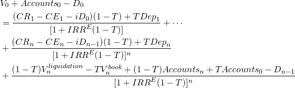
To find rolling NPV, AE, and IRR estimates we divide the numbers in Table 13.4 into acquisition, operating, and liquidation cash flow. We record the acquisition value in all for years in cell N4. We record the ATCF from operations in column M and the ATCF from liquidation in column N. The sum of ATCF from operations and liquidations for the last year of operations is recorded in column O.
Table 13.4. PV Template for
Rolling Estimates of NPV, AE, and IRR for Equity Invested in Green
and Clean Services (GCS)
Open Table 13.4 in Microsoft Excel
| A | B | C | D | E | F | G | H | I | J | K | L | M | N | O | P | Q | R | |
| 3 | Yr | Capital accounts values | Debt Capital | Capital accounts liquidation value | Capital accounts book value | Operating accounts values (AR- INV – AP – AL) | Capital Accounts Depr. | Cash Receipts (CR) | Cash Cost of Goods Sold (COGS) | Cash Overhead Expenses (OE) | Interest Costs | Tax savings from depr. (TxDepr) | After-tax cash flow (ATCF) from operations | ATCF from liquidating Capital and operating accounts | ATCF from operations and liquidations | Rolling NPV | Rolling AE | Rolling IRR |
| 4 | 0 | $40,000 | $10,000 | $40,000 | $0 | $30,000 | $30,000 | |||||||||||
| 5 | 1 | $0 | $9,000 | $30,000 | $30,000 | $1,000 | $10,000 | $19,000 | $9,000 | $0 | $600 | $4,000 | $9,640 | $20,600 | $30,240 | ($1,471.70) | ($1,471.70) | 0.80% |
| 6 | 2 | $0 | $8,000 | $20,000 | $15,000 | $1,200 | $15,000 | $29,800 | $13,500 | $0 | $540 | $6,000 | $15,456 | $9,720 | $25,176 | $1,500.89 | $750.44 | 9.07% |
| 7 | 3 | $0 | $7,000 | $15,000 | $5,000 | $800 | $10,000 | $36,400 | $16,200 | $0 | $480 | $4,000 | $15,832 | $3,480 | $19,312 | $9,064.85 | $3,021.62 | 19.89% |
| 8 | 4 | $0 | $6,000 | $10,000 | $0 | $400 | $5,000 | $40,400 | $18,000 | $0 | $420 | $2,000 | $15,188 | -$760 | $14,428 | $17,571.30 | $4,392.83 | 27.80% |
In the IRR tab we record the ATCF for each year of possible economic life. In our case the ATCF for years 1,2,3, and 4 are recorded in columns B, C, D, and E. In the IRR tab in rows 8, 9, and 10 we report NPV, AE, and IRR for each year and repeat them for convenience in columns P, Q, and R in Table 13.5.
Table 13.5. ATCF, NPV, AE,
and IRR for GCS for economic lives of 1, 2, 3, and 4 years for
equity of $30,000 invested in GCS.
Open Table 13.5 in Microsoft Excel
| A | B | C | D | E | |
| 1 | Economic Life | 1 year | 2 years | 3 years | 4 years |
| 2 | ATFC year 0 (investment) | -$30,000 | -$30,000 | -$30,000 | -$30,000 |
| 3 | ATFC year 1 | $30,240 | $9,640 | $9,640 | $9,640 |
| 4 | ATFC year 2 | $25,176 | $15,456 | $15,456 | |
| 5 | ATFC year 3 | $19,312 | $15,832 | ||
| 6 | ATFC year 4 | $14,428 | |||
| 7 | |||||
| 8 | NPVs | -$1,471.70 | $1,500.89 | $9,064.85 | $17,571.30 |
| 9 | AEs | -$1,471.70 | $750.44 | $3,021.62 | $4,392.83 |
| 10 | IRRs | 0.80% | 9.07% | 19.89% | 27.80% |
Excel Spreadsheets for Describing Exogenous Variable Forecasts
As we increase the sophistication of our forecasts, we recognize the need to use additional Excel spreadsheets identified by tabs. These describe the procedures we followed to estimate the future values of exogenous variables and the values of exogenous variables we estimated. The tabs appear at the bottom of Tables 13.2 that we describe next. Similar tabs describe the exogenous variable projection procedures and values for Table 13.4.
Constants tab
After the template tab that contains Table 13.2 and Table 13.4 is the “constants” tab that contains key assumptions employed in the calculation of the Tables 13.2 and 13.4. Although they vary with projection method, they may include such constants as the average federal, state, and local tax rates paid on earnings from the investment or equity earnings, the defenders IRR, growth rate assumptions for debt, liquidation values, CR, COGS, OE and other variables. We represent arbitrary constant value assumption below that would be input to the PV template
Table 13.6a. Excel Template
Constants Worksheet Tab
Open Template in Microsoft Excel
| A | B | |
| 1 | IRRs, tax rates, and growth rates | |
| 2 | defender’s IRR | 10.00% |
| 3 | average tax rate | 20.00% |
| 4 | After-tax rate | 8.00% |
| 5 | average interest rate | 6.00% |
| 6 | debt growth rate | 1.00% |
| 7 | liquid. growth rate | -2.00% |
| 8 | Book value growth rate | -2.00% |
| 9 | acct.bal.growth rate | 1.00% |
| 10 | CR growth rate | 1.00% |
| 11 | COGS growth rate | 1.00% |
| 12 | OEs growth rate | 1.00% |
IRR tab
To calculate IRR required that we assemble ATCF for each PV model with a different term. These along with NPV, AE, and IRR computations we report in the IRR tab. Data for the IRR tab for GCS were reported in Tables 13.3 and 13.5.
Table 13.6b. Excel Template
IRRs Worksheet Tab
Open Template in Microsoft Excel
| A | B | C | D | E | |
| 1 | Economic Life | 1 year | 2 years | 3 years | 4 years |
| 2 | ATFC year 0 (investment) | -$40,000 | -$40,000 | -$40,000 | -$40,000 |
| 3 | ATFC year 1 | $40,800 | $10,000 | $10,000 | $10,000 |
| 4 | ATFC year 2 | $36,000 | $16,040 | $16,040 | |
| 5 | ATFC year 3 | $31,800 | $18,160 | ||
| 6 | ATFC year 4 | $27,240 | |||
| 7 | |||||
| 8 | NPVs | -$2,222.22 | $123.46 | $8,254.84 | $17,449.18 |
| 9 | AEs | -$2,222.22 | $61.73 | $2,751.61 | $4,362.30 |
| 10 | IRRs | 2.00% | 8.19% | 17.15% | 23,46% |
Capital Account tab
The capital account describes the capital investment that is the focus of the investment. Usually, the investment occurs at the beginning of the model, period zero. However, it may describe other investments during the economic life of the analysis.
Table 13.6c. Excel Template
Capital Account Worksheet Tab
Open Template in Microsoft Excel
| A | B | |
| 1 | Capital account value | |
| 2 | $40,000 | -> investment in lawn and snow removal equip |
| 3 | $0 | |
| 4 | 40 |
Liquidation Value of Capital Investments tab
To calculate rolling NPV, AE, and IRR estimates, we must estimate the liquidation value for capital investments. Generally, we treat capital account liquidation values as exogenous. We represent arbitrary projected capital account liquidation values below that would be input to the PV template.
Table 13.6d. Excel Template
Liquidation Value Worksheet Tab
Open Template in Microsoft Excel
| 3 | Yr | Capital accounts values | Capital accounts liquidation value |
| 4 | 0 | $40,000 | |
| 5 | 1 | $0 | $30,000 |
| 6 | 2 | $0 | $20,000 |
| 7 | 3 | $0 | $15,000 |
| 8 | 4 | $0 | $10,000 |
| 9 | 5 | $0 | $10,000 |
| 10 | 6 | $0 | |
| 11 | 7 | $0 |
Book Value of Capital Assets tab
The purchase price of capital assets established a book or accounting value of capital assets. In the CFS, we record the book value of capital assets in firm’s balance sheets. The book value of the firm’s capital assets are adjusted by depreciation rates determined by taxing authorities. There are more than one methods for determining depreciation allowing capital investment owners some flexibility in establishing depreciation amounts. Generally, the time value of money encourages investment owners to depreciate their investments as rapidly as possible. In this tab, we generally describe the depreciation method that is used to establish the capital investments’ book values. We represent arbitrary projected book values of capital accounts below that would be input to the PV template.
Table 13.6e. Excel Template
Book Value Worksheet Tab
Open Template in Microsoft Excel
| A | |
| 1 | Capital Accounts Book Value |
| 2 | $40,000 |
| 3 | $30,000 |
| 4 | $15,500 |
| 5 | $5,000 |
| 6 | $0 |
| 7 | $0 |
Depreciation Rate tab
The Excel spreadsheet that corresponds to the depreciation rate tab (Dep) describes the depreciation method applied to the capital investments to determine their book value. This tab most often includes the depreciation base for capital investments so that multiplying the depreciation rates times the base calculates the depreciation amount in each year. We represent arbitrary projected depreciation values below that would be input to the PV template
Table 13.6f. Excel Template
Depreciation Worksheet Tab
Open Template in Microsoft Excel
| A | B | C | D | |
| 1 | Year | Depr. Base | Depr. Rate | Depr. Amount |
| 2 | 0 | $40,000 | ||
| 3 | 1 | 25% | $10,000 | |
| 4 | 2 | 37.50% | $15,000 | |
| 5 | 3 | 25% | $10,000 | |
| 6 | 4 | 12.50% | $5,000 | |
| 7 | 5 | 0% | 0 |
Sum of Operating Accounts tab
Increases in the sum of operating accounts (AR+Inv) represent income not received as cash. Decreases in the sum of operating accounts (AR+Inv) represent income earned previously received as cash in the current period. Increases in the sum of operating accounts (AP+AL) represent expenses not paid for in cash. Decreases in the sum of operating accounts (AP+AL) represent expenses incurred previously paid in the current period. The sum of operating accounts are reported in this tab. We represent arbitrary projected sums of operating accounts below that would be input to the PV template.
Table 13.6g. Excel Template
Operating Accounts Worksheet Tab
Open Template in Microsoft Excel
| B | C | D | E | F | |
| 1 | AR | INV | AP | AL | Op. Acc. Sum |
| 2 | 1640 | 3750 | 3000 | 958 | 1432 |
| 3 | 1200 | 5200 | 4000 | 880 | 1520 |
| 4 | 1550 | ||||
| 5 | 1580 | ||||
| 6 | 1610 | ||||
| 7 | 1500 |
Cash Receipts tab
Cash receipts are the oxygen of the firm and investment. We might say that cash receipts are the sine qua non tab because without it nothing else exists for long. In addition, we might also claim that it is the leading exogenous variable because other cash flow variables such as COGS and OE are related to it. Finally, it is the variable most often the focus on professional forecasts or at least the focus of variables highly correlated with CR such as prices. We will have more to say about the Excel sheet that correspond to the CR tab later on. We represent arbitrary projected cash CR estimates below that would be input to the PV template.
Table 13.6h. Excel Template
Cash Receipts Worksheet Tab
Open Template in Microsoft Excel
| A | B | |
| 1 | Cash Receipts | |
| 2 | Year | |
| 3 | 0 | $19000.00 |
| 4 | 1 | $19190.00 |
| 5 | 2 | $19381.90 |
| 6 | 3 | $19575.72 |
| 7 | 4 | $19771.48 |
| 8 | 5 | $19969.19 |
Cash COGS tab
Cash COGS follow closely CR values since by definition they are the costs that vary with production. Therefore, most forecasts of Cash COGS use CR as a variable in the COGS forecast. COGS forecasts may also benefit from projections of input prices. We represent arbitrary projected cash COGS estimates below that would be input to the PV template.
Table 13.6i. Excel Template
COGS Worksheet Tab
Open Template in Microsoft Excel
| A | B | |
| 1 | Cost of Goods Sold | |
| 2 | Year | |
| 3 | 0 | |
| 4 | 1 | $9,000.00 |
| 5 | 2 | $9,090.00 |
| 6 | 3 | $9,180.90 |
| 7 | 4 | $9,272.709 |
| 8 | 5 | $9,365.436 |
Cash OE tab
Cash OE may be related to CR but less so than cash COGS. The initial value for OE may be determined by the size of the business and production activity but in later periods overhead expenses may be less tied to production that input prices that vary over time. Therefore, we sometimes estimate cash OE based on their previous period’s value plus some function of time designed to capture changes in utility, labor, and general maintenance costs. We represent arbitrary projected OE estimates below that would be input to the PV template.
Table 13.6j. Excel Template
Cash OE Worksheet Tab
Open Template in Microsoft Excel
| A | B | |
| 1 | Cash Overhead Expenses | |
| 2 | Year | |
| 3 | 0 | |
| 4 | 1 | $300.00 |
| 5 | 2 | $305.00 |
| 6 | 3 | $310.00 |
| 7 | 4 | $315.00 |
| 8 | 5 | $320.00 |
More Sophisticated Forecasts for GCS
Multi-period PV models depend on forecasts of future values of exogenous variables. Our forecasts of exogenous variables differ in their sophistication and resources committed to their estimation. Obviously, we can never validate our forecasts until the time of the forecast has passed, leading us to infrequently report the accuracy of our predictions—which are usually “wide of the mark”.
So as the quip goes, if you cannot guess correctly, guess often! That strategy is exactly what we recommend here: make frequent forecast updates as new information becomes available. We begin with a base forecast, the one we expect most likely to occur. In our case, we reported the base forecasts for GCS in Tables 13.2 and 13.4. Then we make additional forecasts employing a variety of methods and resources.
Status quo
We begin with the least sophisticated forecast—that the future will be the same as the present. The rational for this approach is that our best forecast is likely the closest to the present. In our case, we assume future CR and COGS in period one continue for the next four years and that AR remain at $1,000. We continue with our other assumptions and resolve the PV template for investments. We describe the results in Table 13.7.
Table 13.7. PV Template for
Rolling Estimates of NPV, AE, and IRR for Green and Clean Services
(GCS) Assuming Constant CR and COGS
Open Template in Microsoft Excel
| A | B | C | D | E | F | G | H | I | J | K | L | M | N | O | P | |
| 3 | Yr | Capital accounts values | Capital accounts liquidation value | Capital accounts book value | Operating accounts values (AR + INV – AP – AL) | Capital Accounts Depr. | Cash Receipts (CR) | Cash Cost of Goods Sold (COGS) | Cash Overhead Expenses (OE) | Tax savings from depr. (TxDepr) | After-tax cash flow (ATCF) from operations | ATCF from liquidating capital and operating accounts | ATCF from operations and liquidations | Rolling NPV | Rolling AE | Rolling IRR |
| 4 | 0 | $40,000 | $40,000 | $0 | $40,000 | $40,000 | ||||||||||
| 5 | 1 | $0 | $30,000 | $30,000 | $1,000 | $10,000 | $19,000 | $9,000 | $0 | $2,000 | $10,000 | $30,800 | $40,800 | ($2,222.22) | ($2,222.22) | 2.00% |
| 6 | 2 | $0 | $20,000 | $15,000 | $1,000 | $15,000 | $19,000 | $9,000 | $0 | $3,000 | $11,000 | $19,800 | $30,800 | ($4,334.71) | ($2,167.35) | 1.14% |
| 7 | 3 | $0 | $15,000 | $5,000 | $1,000 | $10,000 | $19,000 | $9,000 | $0 | $2,000 | $10,000 | $13,800 | $23,800 | ($2,416.81) | ($805.60) | 5.07% |
| 8 | 4 | $0 | $10,000 | $0 | $1,000 | $5,000 | $19,000 | $9,000 | $0 | $1,000 | $9,000 | $8,800 | $17,800 | ($288.16) | ($72.04) | 7.70% |
| 9 | 5 | $0 | $10,000 | $0 | $1,000 | $0 | $19,000 | $9,000 | $0 | $0 | $8,000 | $8,800 | $16,800 | $4,677.38 | $935.48 | 12.06% |
We can observe these consequences of our more conservative growth assumptions. NPV and AE remain negative throughout the four years. Only in the fifth year does the IRR exceed the after-tax discount rate of 8% turning NPV and AE positive. The IRR for GCS is increasing and we expect that by year five will exceed the after-tax IRR of the defender. Contributing to the positive NPV in period five is the liquidation of the capital accounts that Lon assumes will be the same value as in year four.
Constant percentage change assumptions
Next in forecast sophistication, we assume a constant growth
(decay) rate assumption about CR and COGS. In this forecast we
project  and similarly we project COGS as:
  .Our
assumptions for gCR and
gCOGS we describe in the Excel sheet accessed
through the constant tab—each assumed to equal 1%. We project the
future values for CR and COGS and report them in the Excel sheets
reference by the CR and COGS tabs. Then we copy them into the GCS
investment template and report the results in Table 13.8.
.Our
assumptions for gCR and
gCOGS we describe in the Excel sheet accessed
through the constant tab—each assumed to equal 1%. We project the
future values for CR and COGS and report them in the Excel sheets
reference by the CR and COGS tabs. Then we copy them into the GCS
investment template and report the results in Table 13.8.
Table 13.8. PV Template for
Rolling Estimates of NPV, AE, and IRR for Green and Clean Services
(GCS) Assuming Constant % Δ in CR and COGS
Open Table 13.8 in Microsoft Excel
| A | B | C | D | E | F | G | H | I | J | K | L | M | N | O | P | |
| 3 | Yr | Capital accounts values | Capital accounts liquidation value | Capital accounts book value | Operating accounts values (AR + INV – AP – AL) | Capital Accounts Depr. | Cash Receipts (CR) | Cash Cost of Goods Sold (COGS) | Cash Overhead Expenses (OE) | Tax savings from depr. (TxDepr) | After-tax cash flow (ATCF) from operations | ATCF from liquidating capital and operating accounts | ATCF from operations and liquidations | Rolling NPV | Rolling AE | Rolling IRR |
| 4 | 0 | $40,000 | $40,000 | $0 | $40,000 | $40,000 | ||||||||||
| 5 | 1 | $0 | $30,000 | $30,000 | $1,000 | $10,000 | $19,000 | $9,000 | $0 | $2,000 | $10,000.00 | $30,800 | $40,800 | ($2,222.22) | ($2,222.22) | 2.00% |
| 6 | 2 | $0 | $20,000 | $15,000 | $1,000 | $15,000 | $19,190 | $9,090 | $0 | $3,000 | $11,080.00 | $19,800 | $30,880 | ($4,266.12) | ($2,133.06) | 1.25% |
| 7 | 3 | $0 | $15,000 | $5,000 | $1,000 | $10,000 | $19,382 | $9,181 | $0 | $2,000 | $10,160.80 | $13,800 | $23,961 | ($2,220.57) | ($740.19) | 5.31% |
| 8 | 4 | $0 | $10,000 | $0 | $1,000 | $5,000 | $19,576 | $9,273 | $0 | $1,000 | $9,242.41 | $8,800 | $18,042 | $86.25 | $21.56 | 8.09% |
| 9 | 5 | $0 | $10,000 | $0 | $1,000 | $0 | $19,771 | $9,365 | $0 | $0 | $8,324.83 | $8,800 | $17,125 | $5,272.86 | $1,054.57 | 12.55% |
Note that increasing CR and COGS by the same percent each period increased the margin between them over time. To illustrate, in year one, (CR – COGS) = ($19,000 – $9,000) = $10,000. In year five, we found the margin to be (CR – COGS) = ($19,771 – $9,365) = $10,406. Because of compounding CR and COGS, NPV turned positive in year four (one year earlier than under the constant value assumption) and the IRR in the constant percentage change model exceeded the IRR in the constant model in each year after the first one.
Linear growth rate assumption
To project linear grow rates is generally a most conservative
assumption that projecting constant percentage growth rates—other
things being equal. There are several different linear assumptions
we can adopt. For example, we might assume that  and
and  where t = 1, 2, 3, 4, 5 and constants
  and
and  .
We project the future values for CR and COGS using our estimating
and report them in the Excel sheets reference by the CR and COGS
tabs. Then we copy them into the GCS investment template and report
the results in Table 13.9.
.
We project the future values for CR and COGS using our estimating
and report them in the Excel sheets reference by the CR and COGS
tabs. Then we copy them into the GCS investment template and report
the results in Table 13.9.
Table 13.9. PV Template for
Rolling Estimates of NPV, AE, and IRR for Green and Clean Services
(GCS) Assuming Linear Δ in CR and COGS
Open Table 13.9 in Microsoft Excel
| A | B | C | D | E | F | G | H | I | J | K | L | M | N | O | P | |
| 3 | Yr | Capital accounts values | Capital accounts liquidation value | Capital accounts book value | Operating accounts values (AR + INV – AP – AL) | Capital Accounts Depr. | Cash Receipts (CR) | Cash Cost of Goods Sold (COGS) | Cash Overhead Expenses (OE) | Tax savings from depr. (TxDepr) | After-tax cash flow (ATCF) from operations | ATCF from liquidating capital and operating accounts | ATCF from operations and liquidations | Rolling NPV | Rolling AE | Rolling IRR |
| 4 | 0 | $40,000 | $40,000 | $0 | $40,000 | $40,000 | ||||||||||
| 5 | 1 | $0 | $30,000 | $30,000 | $1,000 | $10,000 | $19,000 | $9,000 | $0 | $2,000 | $10,000 | $30,800 | $40,800 | ($2,222.22) | ($2,222.22) | 2.00% |
| 6 | 2 | $0 | $20,000 | $15,000 | $1,000 | $15,000 | $19,100 | $9,110 | $0 | $3,000 | $10,992 | $19,800 | $30,792 | ($4,341.56) | ($2,170.78) | 1.12% |
| 7 | 3 | $0 | $15,000 | $5,000 | $1,000 | $10,000 | $19,200 | $9,330 | $0 | $2,000 | $9,896 | $13,800 | $23,696 | ($2,506.22) | ($835.41) | 4.96% |
| 8 | 4 | $0 | $10,000 | $0 | $1,000 | $5,000 | $19,300 | $9,660 | $0 | $1,000 | $8,712 | $8,800 | $17,512 | ($589.27) | ($147.32) | 7.39% |
| 9 | 5 | $0 | $10,000 | $0 | $1,000 | $0 | $19,400 | $10,100 | $0 | $0 | $7,440 | $8,800 | $16,240 | $3,995.14 | $799.03 | 11.51% |
Projections based on related forecasts
To this point, we have projected CR and COGS based on their past values and time. Most sophisticated projections take advantage of expert predictions based on observed value of related variables in the past. Suppose that for the last seven years, prices of lawn care and snow removal services were $13, $12, $13.5, $15, $16, $18, $17.5, and $17.9 for t = 0, 1, 2, 3, 4, 5, 6, 7. We project future prices p for t = 8, 9, 10, 11, 12, 13 for lawn care and snow removal services using Excel’s forecast option.
Table 13.10. Excel Forecast
Estimate
Open Template in Microsoft Excel
| A | B | C | D | E | |
| 1 | time | observed | Forecast(observed) | Lower Confidence Bound(observed) | Upper Confidence Bound(observed) |
| 2 | 0 | 13 | |||
| 3 | 1 | 12 | |||
| 4 | 2 | 13.5 | |||
| 5 | 3 | 15 | |||
| 6 | 4 | 16 | |||
| 7 | 5 | 18 | |||
| 8 | 6 | 17.5 | |||
| 9 | 7 | 17.9 | 17.90 | 17.90 | 17.90 |
| 10 | 8 | 19.73214458 | 17.99 | 21.47 | |
| 11 | 9 | 21.59962998 | 19.81 | 23.39 | |
| 12 | 10 | 21.62645857 | 19.78 | 23.47 | |
| 13 | 11 | 22.85993116 | 20.96 | 24.76 | |
| 14 | 12 | 24.72741656 | 22.78 | 26.68 | |
| 15 | 13 | 24.75424515 | 22.75 | 26.75 |
Figure 13.3. Graph of
Projection Estimates
Open Template in Microsoft Excel
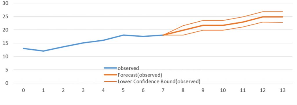
Having obtained price forecasts, our next step would be to re-estimate CR for GCS based on the forecasted prices. In addition, we may use the confidence interval forecasts to find a most optimistic forecast using the upper confidence interval forecasts and a pessimistic forecast using the lower bound forecasts.
The forecasts above have been presented as coming from a “black box”. The black box, in this case contains well-known statistical methods that can easily be learned but beyond an already over ambitious collection of topics covered in this book.
Incremental Investments
Incremental investments may replace, modify, or expand an existing investment. Regardless, the incremental investment analysis approach is the same: it compares the defending investment with changes that result from an incremental investment. What is common to incremental investments is that something of the original investment remains.
In what follows, we illustrate an incremental investment with a bakery considering replacing its doughnut-making machine. Other investments supporting the doughnut making machine are assumed to be unaffected by the incremental investment.
Brown and Round Doughnuts
We next consider two alternative machines for making doughnuts. One machine is the one already in operation. In this case the challengers are an older version of the original machine and a new machine. Should you continue with the used machine, buy a new machine, or get out of the doughnut business?
Continuing to make doughnuts with the old machine.
In this example the challenger is an older version of the original investment. To be specific, suppose you bought a doughnut machine 3 years ago for $90,000. You are depreciating the machine over 5 years using the MACRS method, and the expected market value 5 years from today is $10,000. The machine generates $30,000 in cash revenues and produces $15,000 in cash expenses each year. If you sold the machine today, you could get $30,000 from a local competitor.
Your after-tax ROA-IRR, r(1 – T), is 10%, your marginal tax rate is 40%, and the capital gains tax is 20%. Assume book value depreciation can be used to offset ordinary income.
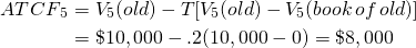
Let’s begin with the old machine. Keeping the old machine is equivalent to reinvesting its $30,000 current value (V0) in the business and forfeiting the tax refund from capital losses. To determine the tax refund forfeited, recall that the used machine was purchased 3 years earlier for $90,000, and has been depreciated using 5-year MACR, so the machine’s book value is $90,000(100% – 15% – 25.5% –17.85%) = $37,485.
Since book value exceeds liquidation value, a tax
credit is owed to the seller equal to  Now we can write the acquisition ATCF as
  = – $30,000 – $2,994 = –$32,994. Finally, 5 year MACR depreciation
rates on the old machine equal: 16.66%, 16.66%, and 8.33%. We write
the ATCF for the tth period as:
= – $30,000 – $2,994 = –$32,994. Finally, 5 year MACR depreciation
rates on the old machine equal: 16.66%, 16.66%, and 8.33%. We write
the ATCF for the tth period as:
(13.11)
However, because ATCF per period differs, we describe it using Table 13.11. below.
Table 13.11. Finding ATCF for Continuing to Operate with the Old Doughnut Machine
| Old Doughnut Machine Operating ATCF | ||||||
| Year | CRt | CEt |
Dept |
(CRt – CEt)(1– T) + T Dept |  |
ATCF1 |
| 1 | 30,000 | 15,000 |
14,994 (16.66%) |
(15,000 x .6) + (14,994 x .4) = 14,998 | 0 | $14,998 |
| 2 | 30,000 | 15,000 |
14,994 (16.66%) |
(15,000 x .6) + (14,994 x .4) = 14,998 | 0 | $14,998 |
| 3 | 30,000 | 15,000 |
7,470 (8.33%) |
(15,000 x .6) + (7470 x .4) = 11,988 | 0 | $11,988 |
| 4 | 30,000 | 15,000 | 0 | (15,000 x .6) = 9,000 | 0 | $9,000 |
| 5 | 30,000 | 15,000 | 0 | (15,000 x .6) = 9,000 | 0 | $9,000 |
Finally, we write the salvage value for the old machine. Recalling that the salvage value of the old machine, V5, is $10,000, that the old machine is completely depreciated, and the capital gains tax rate Tg is 0.2, we can write the salvage value as:
(13.12)
Finally, we are prepared to combine the ATCF from the acquisition, operation, and liquidation of the old doughnut machine. We express these in Table 13.12.
Table 13.12. Old Doughnut Machine Operating ATCF
| Year | CRt | CEt |
Dept (MACR) |
(CRt – CEt)(1– T) + T Dept | |
ATCF1 |
| 0 | –V0 – T(V0 – V0book) = –$30,000 – (.4)($30,000 – $37,485) = – $30,000 – $2,994 = –$32,994 |
–$32,994 |
||||
| 1 | 30,000 | 15,000 |
14,994 (16.66%) |
(15,000 x .6) + (14,994 x .4) = 14,998 | 0 | $14,998 |
| 2 | 30,000 | 15,000 |
14,994 (16.66%) |
(15,000 x .6) + (14,994 x .4) = 14,998 | 0 | $14,998 |
| 3 | 30,000 | 15,000 |
7,470 (8.33%) |
(15,000 x .6) + (7470 x .4) = 11,988 | 0 | $11,988 |
| 4 | 30,000 | 15,000 | 0 | (15,000 x .6) = 9,000 | 0 | $9,000 |
| 5 | 30,000 | 15,000 | 0 | (15,000 x .6) = 9,000 | 0 | $9,000 |
| 5 | V5 – T(V5 – V5book) = $10,000 – (.2)($10,000 – 0) = $10,000 – $2,000 = $8,000 | $8,000 (Liquidation) |
||||
The only other calculation left is to compute the NPV of the old doughnut machine which we complete using our Excel spreadsheet.
Table 13.13. Old Doughnut
Machine
Open Table 13.13 in Microsoft Excel
| A | B | C | |
| 1 | Old Doughnut Machine | ||
| 2 | variables | data | formulas |
| 3 | rate | 0.1 | |
| 4 | Acquisition Cost | ($32,994) | |
| 5 | ATCF1 | $14,998 | |
| 6 | ATCF2 | $14,998 | |
| 7 | ATCF3 | $11,998 | |
| 8 | ATCF4 | $9,000 | |
| 9 | ATCF5 | $9,000 | |
| 10 | Salvage Value | $8,000 | |
| 11 | NPV | $18,745 | “= -V0 + NPV(rate, ATCF1:ATCF5) + Vn / (1 + rate)^5 |
| 12 | IRR | 30% | “=IRR(Acquisition Cost, ATCF1:ATCF5, Salvage Value) |
| 13 | AE | ($4,944.92) | “=PMT(rate, nper, NPV) |
| 14 | nper | 5 | |
Purchasing a new doughnut machine.
Assume that, after completing the PV analysis of the old doughnut machine, a salesman for a “new and improved” doughnut machine stops by and wants to sell you a new machine. The new machine will increase your revenues to $45,000 each year, and decrease your expenses to only $10,000 each year. The new machine costs $90,000 and will require $10,000 for delivery and installation costs. Thus, the acquisition ATCF0 = $100,000. The machine will fall into the MACRS five-year depreciation class (15%, 25.5%, 17.85%, 16.66%, 16.66%, and 8.33%). The machine is expected to have a $40,000 salvage value after 5 years.
Next, we need to determine the operating ATCF for the new machine. Tax rates, the defender’s after-tax IRR, and MACR depreciation rates are the same as before—equal to those used to evaluate the continued use of the old doughnut machine. Because of the level of sales, accounts receivable and accounts payable increase by $5,000 and $2,000 in the first year respectively. They are reduced by the same amount in the fifth year. The formula for operating ATCF is the same as before except that sales and expenses are no longer just cash items and must be adjusted by the term ∆Vn = ∆CA – ∆CL = $5,000 – $2,000 = $3,000
(13.13)

The new machine will be depreciated using the 5-year MACRS method. The depreciation for each machine, and the change in depreciation each year for the next 5 years is:
Table 13.14a. New Doughnut Machine Depreciation
| Year | $100,000 x MACR rate | = | Depreciation |
| 1 | $100,000 x 15% | = | $15,000 |
| 2 | $100,000 x 25.5% | = | $25,500 |
| 3 | $100,000 x 17.85% | = | $17,850 |
| 4 | $100,000 x 16.66% | = | $16,660 |
| 5 | $100,000 x 16.66% | = | $16,660 |
Remember that depreciation expense is a noncash expense, which by itself doesn’t generate a cash flow. However, you can use the depreciation expense to reduce taxable income. As a result, the firm realizes an additional tax savings from depreciation. The amount of the tax savings are described below.
Table 13.14b. New Doughnut Machine Tax Savings
| Year | Tax Savings | = | (Depreciation)(T = .4) |
| 1 | $15,000 x (.4) | = | $6,000 |
| 2 | $25,500 x (.4) | = | $10,200 |
| 3 | $17,850 x (.4) | = | $7,140 |
| 4 | $16,660 x (.4) | = | $6,664 |
| 5 | $16,660 x (.4) | = | $6,664 |
Finally, we find the salvage value as follows. We first recognize that the sale of the doughnut machine in 5 years will increase cash flow by $40,000. Next, we find the asset’s book value in year five as the difference between its acquisition value less its accumulated depreciation: $100,000 – ($15,000 + $25,500 + $17,850 + $16,600 + $16,660) = $8,330. Since the asset’s book value is less than its salvage value, there are capital gains taxes to be paid. Therefore, the salvage value ATCF can be written as the salvage value less the capital gains tax:
(13.14)
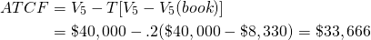
Finally, we combine acquisition, operation, and liquidation ATCF associated with the new doughnut machine in Table 13.15.
Table 13.15. New Doughnut Machine Operating ATCF
| Year | Sales | Expense | Dep. (MACR %) |
(Sales – Expenses) x (1 – T) + T Dep. |
 |
ATCF |
| 0 ATCF0(Acquisition) = –V0 = | –$100,000 | |||||
| 1 ATCF1 | 45,000 | 10,000 |
15,000 (15%) |
(35,000 x .6) + (15,000 x .4) = 27,000 | 3,000 | $24,000 |
| 2 ATCF2 | 45,000 | 10,000 |
25,500 (25.5%) |
(35,000 x .6) + (25,500 x .4) = 31,200 | 0 | $31,200 |
| 3 ATCF3 | 45,000 | 10,000 |
17,850 (17.85%) |
(35,000 x .6) + (17,850 x .4) = 28,140 | 0 | $28,140 |
| 4 ATCF4 | 45,000 | 10,000 |
16,660 (16.66%) |
(35,000 x .6) + (16,660 x .4) = 27,664 | 0 | $27,664 |
| 5 ATCF5 | 45,000 | 10,000 |
16,660 (16.66%) |
(35,000 x .6) + (16,660 x .4) = 27,664 | -3,000 | $30,664 |
| 5 ATCF5 (Liquidation) = V5 – T[V5 – V5(book)] = $40,000 – .2($40,000 – $8,330) = | $33,666 | |||||
We find the NPV for the new doughnut machine in Table 13.16:
Table 13.16. New Doughnut Machine NPV
| Year |  |
ATCF |  |
| 0 | 1 | –$100,000 | –$100,000 |
| 1 | .91 | $24,000 | $21,840 |
| 2 | .83 | $31,200 | $25,896 |
| 3 | .75 | $28,140 | $21,105 |
| 4 | .68 | $27,664 | $18,812 |
| 5 | .62 | $30,664 + $33,666 = $64,330 | $39,885 |
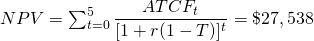 (27,584 using CF worksheet)
 |
|||
Finally, we find the NPV for the new doughnut machine using our Excel Spreadsheet.
Table 13.17. New Doughnuts
Machine
Open Table 13.13 in Microsoft Excel
| A | B | C | |
| 1 | New Doughnut Machine | ||
| 2 | variables | data | formulas |
| 3 | rate | 0.1 | |
| 4 | Acquisition Cost | ($100,000) | |
| 5 | ATCF1 | $24,000 | |
| 6 | ATCF2 | $31,200 | |
| 7 | ATCF3 | $28,140 | |
| 8 | ATCF4 | $27,664 | |
| 9 | ATCF5 | $30,664 | |
| 10 | Salvage Value | $33,666 | |
| 11 | NPV | $27,584 | “= -V0 + NPV(rate, ATCF1:ATCF5) + Vn / (1 + rate)^5 |
| 12 | IRR | 18% | “=IRR(Acquisition Cost, ATCF1:ATCF5, Salvage Value) |
| 13 | AE | ($7,276.60) | “=PMT(rate, nper, NPV) |
| 14 | nper | 5 | |
The result of the analysis is that NPV will be positive for both options by continuing to use the old machine or by investing in the new one. However, the firm’s NPV will increase the most if it adopts the new machine—an increase of $8,839 ($27,584 – $18,745) over continuing to use the old machine. However, the IRR of the old machine is greater, and we have a conflict between IRR and NPV rankings. The ranking is resolved by deciding on the reinvestment rate for the differences in funding required by the two investments. If the difference in funding levels is invested at the discount rate, the NPV rankings are appropriate. If the investments can be scaled, then the IRR rankings are appropriate. It is assumed here that the reinvestment rate is the after-tax IRR of the defender, 10%, so that any differences in size would not change their respective NPVs, and NPV rankings are appropriate.
Summary and Conclusions
This chapter operationalized PV analysis by introducing two PV multi-period templates, one for analysis of investments and the second one for analysis of equity committed to investments. In this effort we adjusted the average tax rate to correspond to the average tax rate paid on investments versus the average tax rate paid on equity committed to investments.
We reached an important conclusion when we analyzed returns on investments (assets) and equity. They need not rank investments and equity committed to investment consistently. These results add you our earlier finding that NPV and IRR models need not rank investments consistently homogeneous size and term conditions are satisfied.
That returns on investments and equity committed to investments may produce inconsistent ranking leads to an important question: when should we rank investment using returns on investments (assets) versus returns on equity committed to investments? The general answer is: it depends on who is asking. An individual investor whose financial conditions including loan amounts and costs are likely to be most interested in knowing returns to his/her specific conditions. Those more interested in the general condition of an industry or class of investments will more likely be most interested in returns on the investment or class of firms.
Not only have we focused on analyzing firms and investments versus returns on equity invested in firm’s and investments, we have also focused on the analysis of stand-alone versus incremental investments. In Chapter 12 we used accrual income statement (AIS) to find rates on return on assets and equity for a firm. The analysis was for a single period and focused primarily on describing the condition of the firm. In contrast, this chapter has focused on investments that add to, alter, or replace firm investments. We referred to investments that add to, replace, or change the firm’s capital structure as incremental investments. Sometimes the language used to describe incremental investments is confusing and describes them as partial budgeting analysis. We may use partial budgets to describe an incremental investment—but should not be confused with the actual PV analysis of incremental investments.
An irony is that most often practical applications of PV analysis are focused on stand-alone investments while most practical investments are incremental ones. Included in this irony is that tax rates most often refer to equity commitments rather than investment commitments.
To illustrate PV analysis, we focused on two practical investments. One a stand-alone investment we referred to as Green and Clean Services (GCS) and the second, an incremental investment we referred to as Round and Brown Doughnuts. In the first case we focused on how to distinguish between investment versus equity committed to investment analysis. The important point is this example was how the financial terms of the loan can change the attractiveness of the investment and, of course, change the rankings between investments.
When conducting PV analysis and making prescriptive statements based on the analysis, we have to estimate the future. Of course, some may argue that this involves sophisticated guessing—or estimating as some would refer to the efforts. Estimates of the future range in their sophistication—but they have one thing is common, they are never completely accurate. To remedy this problem, we recommend analyzing one’s investment and equity committed to the investment using several different forecasts as illustrated in this chapter and only adopting an investment is the returns are sufficiently positive that we can still be too optimistic in our forecasts and yet earn a comfortable rate of return.
PV analysis and forecasting the future is an important and unavoidable task. Hopefully, the tools described in this chapter will aid in that effort.
Questions
- Please describe the difference in investment focus between an AIS and a PV model?
- What is the main difference between a stand-alone versus an incremental investment? Explain why some sources describe incremental investment analysis as partial budgeting analysis.
- This chapter presented two main PV model templates. One focused on analyzing investments. The second one focused on analyzing equity committed to the investment. Describe the differences between the two templates. Then explain how these differences permit us to calculate returns associated with investments versus returns on equity committed to investments.
- Describe the nature of a fixed investment.
- A capital investment provides services over several periods. A nondurable provides services once. Explain how this difference in capital goods and nondurable inputs are recognized in PV models.
- A capital investment provides services for more than one period without losing its identity. The cost of providing these services is the change in the liquidation of the capital asset and the use of nondurable goods. The change in the liquidation value of a capital asset may mostly depend on the passage of time and the intensity of its use. Please explain how these two costs that result from the passage of time an use influence the optimal service extraction rate from the capital asset.
- Operating accounts include AR, INV, AP, and AL. Describe how decreases (increases) in capital accounts influence operating and liquidation ATCF.
- What is the difference between exogenous and endogenous variables used to solve for NPV, AE, and IRR in PV models?
- Solving PV models requires that we forecast the values of exogenous and endogenous variables for the economic life of the investment. Describe how these forecasts might vary in their sophistication.
- Assume you are attending school, working part time, and need transportation. To satisfy your transportation needs, you consider three options: You could continue driving your old clunker. You could buy a new car. Alternatively, you could buy a newer used car.
Your parents, who will need to loan you the money if you buy a new or newer used car, prefer that you continue to drive your clunker. You have done your homework to determine which of the three transportation options is the least cost one—although there may be other considerations. The financial data for the three investments follows.
Continue driving the clunker. You list the following financial details associated with continuing to drive the clunker. The clunker’s current market value is V = $3,000 which is the amount that you would sacrifice if you keep the clunker. As a result, you consider it to be your acquisition price. You estimate that you will travel 1,000 miles per month for 24 months in the clunker. In addition you estimate repair costs will equal 14 cents per mile, maintenance costs will equal 2.5 cents per mile, fuel costs/mile ($3.00/gallon divided by 17 miles/gallon) will equal 17.6 cents per mile, insurance costs will equal 10 cents per mile, and the clunker’s salvage value in 2 years (24 months) you estimate will equal V24 = $375. The total operating cost per mile for the clunker you estimate to equal 44.1 cents per mile and monthly operating cost you estimate will equal $441.
A new car. It would take a lot of coaxing for your parents to loan you enough money to buy a new car, but you would prefer this option. You can imagine how impressive you would be offering rides to your friends in your new car. You found one that you think would work. The financial characteristics of the new car include an acquisition price of V0 = $24,000, and you estimate that you will travel 1,000 miles per month for 10 years or 120 months in the new car. In addition, you estimate repair costs will equal 3.5 cents per mile, maintenance costs will equal 2.5 cents per mile, fuel costs ($3.00/ gallon divided by 27 miles/gallon) will equal 11.1 cents per mile, insurance costs will equal 12 cents per mile, and the salvage value in 10 years (120 months) you estimate will equal V120 = $8,000 The total operating cost per mile for the new car you estimated will equal 29.1 cents per mile and monthly operating costs you estimate will equal $291.
A used car. In case you cannot get the loan to buy a new car, you consider a newer used car to be an acceptable alternative to continuing to drive your clunker. You found one that you think would work. The financial characteristics include an acquisition price of V0 = $19,800, and you estimate that you will travel 1,000 miles per month for 8 years or 96 months in the newer used car. You estimate repair costs will equal 5 cents per mile, maintenance costs will equal 2.5 cents per mil, fuel costs ($3.00/gallon divided by 21.4 miles/gallon) will equal 14 cents per mile, insurance costs will equal 11 cents per mile, and the salvage value in 8 years (96 months) you estimate will equal V96 = $7,000 The total operating cost per mile for the used car you estimate will equal 32.5 cents per mile and you estimate monthly operating costs will equal $325.
Summary of data. We summarize the financial characteristics of the three car options in the Table Q13.1 below. Included in the table are the three phases of the investment: the acquisition costs, the operating costs per month, and the salvage values. Note that the operating costs are lowest for the new car. The acquisition cost is lowest for the clunker. Not included in the Table Q13.1 data summary is the average value of the investment lost per year—the average depreciation cost. We find the average depreciation cost by subtracting from the acquisition value the liquidation value and this difference we divide by the number of service months. This cost is ($3,000 –$ 375) / 24 = $109.38 for the clunker, ($24,000 – $8,000) / 120 = $133.3 3 for the new car, and ($19,800 – $7,000) / 96 = $133.33 for the used car. Since we account for these costs as the acquisition and liquidation values, they are not included in our monthly costs. We note, however, that one significant advantage of the clunker is its lower monthly depreciation.
Table Q13.1. A summary of per mile and monthly costs of driving a clunker, a new car, and a used car.
| Clunker | New Car | Used Car | |
| – V0 | $3,000 | $24,000 | $19,800 |
| Miles driven per month | 1,000 | 1,000 | 1,000 |
| Repair costs per mile | $0.14 | $0.035 | $0.05 |
| Maintenance costs per mile | $0.025 | $0.025 | $0.025 |
| Miles per gallon | 17 | 27 | 25 |
| Fuel cost per mile ($3 / gal) | $3 / 17 = $0.176 | $3 / 27 = $0.111 | $3 / 25 = $0.12 |
| Insurance cost per mile | $0.10 | $0.12 | $0.11 |
| Total operating cost per mile | $0.441 | $0.291 | $0.325 |
| Operating cost per
month (1000 miles/month * cost/mile) |
$441 | $291 | $325 |
| Economic life (months) | 24 | 120 | 96 |
| Salvage Value (Vn) | V24 = $375 | V120 = $8,000 | V96 = $7000 |
| Interest rate per year / month | 12% / 1% | 12% / 1% | 12% / 1% |
Net present cost (NPC). Your goal is to select the least cost transportation option. What makes this problem especially interesting is that the term is different for each car option requiring that we compare car transportation costs using their annuity equivalent (AE) cost per month. Your assignment is to find the NPC, AE, and IRR for the useful life of each car using the template that corresponds to equation 13.21 with T set equal to zero. Then describe your rankings.