
5: Financial Ratios
- Page ID
- 12750

After completing this chapter, you should be able to: (1) calculate financial ratios using information included in a firm’s coordinated financial statements (CFS); and (2) answer the question: “what are the firm’s financial strengths and weaknesses?”
To achieve your learning goals, you should complete the following objectives:
- Learn how to interpret ratios.
- Learn how financial ratios allow us to compare the financial condition of different firms.
- Learn how to construct (S)olvency, (P)rofitability, (E) fficiency, (L)iquidity, and (L)everage ratios—what we refer to collectively as SPELL ratios.
- Learn how SPELL ratios help us describe the financial strengths and weaknesses of a firm.
- Learn how the times interest earned (TIE) ratio and the debt-to-service (DS) ratio can provide information about the firm’s solvency.
- Learn how the profit margin (m) ratio, the return on assets (ROA) ratio, and the return on equity (ROE) ratio can provide information about the firm’s profitability.
- Learn how to find the after-tax ROE where T is the average tax rate paid by the firm on its earnings before taxes (EBT).
- Learn how to relate ROE and ROA to each other.
- Learn how the inventory turnover (ITO) ratio, the inventory turnover time (ITOT) ratio, the asset turnover (ATO) ratio, the asset turnover time (ATOT) ratio, the receivable turnover (RTO) ratio, the receivable turnover time (RTOT) ratio, the payable turnover (PTO) ratio, and the payable turnover time (PTOT) ratio can provide important efficiency information about the firm.
- Learn how the current ratio (CT) and the quick ratio (QK) can provide information about the firm’s liquidity.
- Learn how leverage ratios including the debt-to-equity (DE) ratio and the equity multiplier (EM) ratio can be used to monitor and measure the firm’s risk.
- Understand how comparing the firm’s SPELL ratios to industry standard ratios can help answer the question: what are the financial strengths and weaknesses of the firm?
- Learn how to construct after-tax ROE and after-tax ROA measures.
- Learn how unpaid family labor affects ROE and ROA measures.
- Learn why the firm may consider profit and solvency ratios key to a firm’s survival and success.
- Learn how the DuPont ratio demonstrates the interdependencies of some SPELL ratios.
Introduction
Coordinated financial statement (CFS) variables. CFS contain exogenous and endogenous variables. Exogenous variables take on values that can be observed or are determined by activities occurring outside of the firm. Endogenous variables take on values determined by activities within the firm and the values of exogenous variables.
The variables included in CFS become more valuable, especially for analyzing the strengths and weaknesses of the firm, when formed into ratios. We could look at the variables included in the CFS and draw some conclusions about the firm’s strengths and weaknesses by comparing them with other firms, but our conclusions would be limited because no two firms are alike. Ratios, however, provide a means for comparing the performance of firms using a standardized measure which is easier to interpret.
A ratio consists of two numbers when one number is divided by the other. Suppose two numbers are represented by the variables X and Y and form a ratio (X/Y). The ratio tells us how many units of X exist for each unit of Y. This standardized number, the number of units of X that exists for each unit of Y , allows us to make comparisons between firms using similarly constructed ratios. One other way to interpret the ratio X/Y is to multiply the ratio by 100 converting the ratio to a percentage. In this case the ratio multiplied by 100 tells us what percentage of Y is X.
To illustrate the importance of ratios, consider the purchase of a breakfast cereal. Suppose you go to the grocery store to purchase your favorite breakfast cereal (Super Sweet Sugar Snacks). You find a 10-ounce box of Super Sweet Sugar Snacks that sells for $3.20 and a larger 15-ounce box of the same cereal that sells for $4.50. Which box of cereal is the best buy? The price of each box of cereal won’t tell you the answer because the more expensive box also contains more cereal. However, if we divide the price of each box by the amount of cereal in the box we can compare “apples to apples,” or in this example we can compare the price per ounce of cereal in each box. Finding the ratio of dollars to ounces in the box, we see that cereal in the small box costs $0.32 per ounce ($3.20/10 oz.) while cereal in the large box costs $0.30 per ounce ($4.50/15 oz.). The large box of cereal costs less for each ounce of cereal and is the better buy.
The cereal example illustrates an important fact: one ratio without another ratio to compare it with is not very helpful. Knowing the price of cereal per ounce of the small box makes the information about the price per ounce of cereal in the large box more meaningful. Similarly, having standardized industry ratios against which we can compare our ratios is important for a financial manager’s efforts to discover the firm’s strengths and weaknesses.
We discuss next the different views required to adequately describe the firm’s financial condition. Each of the different views are represented by a set of ratios.
Financial Ratios
Financial ratios constructed using coordinated financial statement variables can be grouped into five categories. The categories can be remembered using the acronym SPELL. The five categories of financial ratios include: (S)olvency ratios, (P)rofitability ratios, (E)fficiency ratios, (L)iquidity ratios, and (L)everage ratios. Ratios in each of these five categories provide a different view of the firm’s financial strengths and weaknesses.
Ratios and points in time measures. When constructing financial ratios using data from the CFS, the “point in time” or the “period of time” reflected by the ratio deserves careful attention. Numbers from balance sheets reflect the financial condition of the firm at a point in time. Numbers from income statements and statements of cash flow describe financial activity over a period of time. When forming a ratio using two numbers from the balance sheet, the numbers should reflect the same point in time.
Ratios of points and period of time measures. There are two approaches when forming a ratio with one number from the income statement or statement of cash flow describing activity over a period of time and another number from the balance sheet reflecting financial conditions at a point in time. One approach uses a number from the previous period’s end of period balance sheet that corresponds with the point in time in which activities reported in the income statement begin. The second approach uses the average of beginning and ending period balance sheet measures that span the period of time during which activities reported in the income statement occurred. Later we will discuss in more detail when each of the two methods is preferred.
Cash versus accrual ratios. We construct several ratios in this chapter that include an income or a COGS variable. The question is: should these be cash receipts and cash COGS or accrued income and accrued COGS? We use accrual variables that focus on when financial transactions occurred rather than when transactions were converted to cash.
Useful comparisons. The usefulness of ratios depends on having something useful to compare them to. Suppose we wish we compare ratios of different firms. Obviously, we would expect ratios constructed for different firms to have been calculated at comparable points and periods of time. We would also expect that firms being compared are of the same size and engaged in similar activities. Fortunately, we can often find such measures described as industry average ratios.
Sometimes the relevant comparison for the firm is with itself at different points in time. Having the same ratio over a number of time periods for the same firm allows the firm manager to identify trends. One question trend analysis may answer is: in what areas is the firm is improving (not improving) compared to past performances. Of course, trend analysis can be performed using absolute numbers as well as ratios.
What follows. In what follows, we will introduce several ratios from each of the five “SPELL” categories. Then we will discuss how each of them, alone and together with other SPELL ratios, can help answer the question: what are the firm’s financial strengths and weaknesses. Since data from HQN’s financial statements will be used to form the SPELL ratios, HQN’s balance sheets, AIS, and statement of cash flow for 2018 are repeated in Table 5.1.
Table 5.1. Coordinated
financial statement for HiQuality Nursery (HQN) for the year
2018
Open HQN Coordinated Financial Statement in MS Excel
| BALANCE SHEET | ACCRUAL INCOME STATEMENT | STATEMENT OF CASH FLOW | ||||||
|---|---|---|---|---|---|---|---|---|
|
12/31/17 |
12/31/18 |
2018 | 2018 | |||||
| Cash and Marketable Securities |
$930 |
$600 |
+ | Cash Receipts | $38,990 | + | Cash Receipts | $38,990 |
| Accounts Receivable |
$1,640 |
$1,200 |
+ | Δ Accounts Receivable | ($440) | – | Cash COGS | $27,000 |
| Inventory |
$3,750 |
$5,200 |
+ | Δ Inventories | $1450 | – | Cash OE | $11,078 |
| Notes Receivable |
$0 |
$0 |
+ | Realized Capital Gains / Depreciation Recapture | $0 | – | Interest paid | $480 |
| CURRENT ASSETS |
$6,320 |
$7,000 |
= | Total Revenue | $40,000 | – | Taxes paid | $68 |
| Depreciable Long-term Assets |
$2,990 |
$2,710 |
+ | Cash Cost of Goods Sold (COGS) | $27,000 | = | Net Cash Flow from Operations | $364 |
| Non-depreciable Long-term Assets |
$690 |
$690 |
+ | Δ Accounts Payable | $1,000 | + | Realized capital gains + depreciation recapture | $0 |
| LONG-TERM ASSETS |
$3,680 |
$3,400 |
+ | Cash Overhead Expenses (OE) | $11,078 | + | Sales non-depreciable assets | $0 |
| TOTAL ASSETS |
$10,000 |
$10,400 |
+ | Δ Accrued Liabilities | ($78) | – | Purchases of non-depreciable assets | $0 |
| Notes Payable |
$1,500 |
$1,270 |
+ | Depreciation | $350 | + | Sales of depreciable assets | $30 |
| Current Portion LTD |
$500 |
$450 |
= | Total Expenses | $39,350 | – | Purchases of depreciable assets | $100 |
| Accounts Payable |
$3,000 |
$4,000 |
Earnings Before Interest and Taxes (EBIT) | $650 | = | Net Cash Flow from Investments | ($70) | |
| Accrued Liabilities |
$958 |
$880 |
– | Interest | $480 | + | Change in noncurrent LTD | ($57) |
| CURRENT LIABILITIES |
$5,958 |
$6,600 |
Earnings Before Taxes (EBT) | $170 | + | Change in current portion of LTD | ($50) | |
| NONCURRENT LONG-TERM DEBT |
$2,042 |
$1,985 |
– | Taxes | $68 | + | Change in notes payable | ($230) |
| TOTAL LIABILITIES |
$8,000 |
$8,585 |
Net Income After Taxes (NIAT) | $102 | – | Payment of dividends and owner’s draw | $287 | |
| Contributed Capital |
$1,900 |
$1,900 |
– | Dividends and owner draws | $287 | = | Net Cash Flow from Financing | ($624) |
| Retained Earnings |
$100 |
($85) |
Additions To Retained Earnings | ($185) | Change in cash position of the firm | ($330) | ||
| TOTAL EQUITY |
$2,000 |
$1,815 |
||||||
| TOTAL LIABILITIES AND EQUITY |
$10,000 |
$10,400 |
||||||
Solvency Ratios
Solvency ratios, sometimes called repayment capacity ratios, can be used to answer questions about the firm’s ability to meet its long-term debt obligations. Here we will examine two solvency ratios: (1) times interest earned (TIE) and (2) debt-to-service ratio (DS).
Times interest earned (TIE) ratio
The TIE ratio measures the firm’s solvency or repayment capacity. The TIE ratio combines two period of time measures obtained from the firm’s income statement and is defined as:
(5.1)
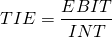
In the above formula, INT represents the firm’s interest obligations accrued during the period. EBIT measures the firm’s earnings during the period before paying interest and taxes. The TIE ratio answers the question: how many times can the firm pay its interest costs using the firm’s operating profits (for every dollar of interest costs how many dollars of EBIT exist? Generally, a healthy firm’s TIE ratio exceeds one (TIE > 1), otherwise the firm won’t be able to pay its interest costs using its current income. HQN’s TIE ratio for 2018 is:
(5.2)
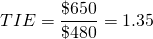
HQN’s 2018 TIE ratio indicates for every dollar of interest the firm owes, it has $1.35 dollars of EBIT to make its interest payments.
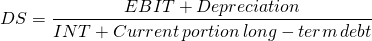
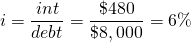
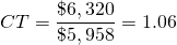
Debt-to-service (DS) ratio
Like the TIE ratio, the DS ratio answers questions about the firm’s ability to pay its current long-term debt obligations. In contrast to the TIE ratio, DS ratio recognizes the need to pay the current portion of its long-term debt in addition to interest. Finally, the DS ratio (in contrast to the TIE ratio) adds depreciation to EBIT because depreciation is a non-cash expense. Subtracting depreciation from revenue to obtain EBIT understates the liquid funds available to the firm to pay its current long-term debt obligations.
To illustrate the logic behind this formula, assume that cash receipts equals $100, depreciation equals $30, other expenses equal $10, and EBIT is equal to $60. But more than $60 is available to pay interest and principal because depreciation of $30 is a non cash expense. Thus we add depreciation to EBIT to improve our measure of income available for interest and debt repayment: $60 + $30 = $90, which is the numerator in the DS ratio equation.
This book recommends that the current portion of the long-term debt at the beginning of the current period be used to calculate the denominator in the firm’s DS ratio. After making these adjustments, we obtain the firm’s DS ratio equal to:
(5.3)
If the DS < 1, a firm will not be able to make principal and interest payments using EBIT plus depreciation. In this case, the firm will be required to obtain funding from other sources such as restructuring debt, selling assets, delaying investments in assets, and/or increasing EBIT to meet current debt and interest obligations. If the firm were unable to meet its interest and principal payment over the long term, the firm’s survival would be threatened.
We can solve for HQN’s 2018 DS ratio. According to HQN’s income statement EBIT was $650 and depreciation was $350. Interest paid equaled $480 and the current portion of the long-term debt listed on the firm’s 2017 end of period balance sheet was $500. Making the substitutions into Equation \ref{5.3} we find HQN’s DS ratio equal to:
(5.4)
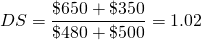
According to HQN’s DS ratio, its EBIT plus depreciation are sufficient to meet 102 percent of its interest and current principal payments, a more accurate reflections of its solvency than its TIE ratio of 1.35.
Profitability Ratios
Profitability ratios measure the firm’s ability to generate profits from its assets or equity. The firm’s accrual income statement (AIS) provides three earnings or profit measures useful in finding rates of return: earnings before interest and taxes (EBIT), earnings before taxes (EBT), and net income after interest and taxes (NAIT).
We examine three profitability ratios: (1) profit margin (m), (2) return on assets (ROA), and (3) return on equity (ROE). In some cases, the profitability measures are reported on an after-tax basis requiring that we know the average tax rate for the firm which we calculate next.
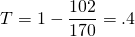
Finding the average tax rate. In some cases, particularly with profitability measures, we need to know the average tax rate paid by the firm. We find the average tax rate by solving for T in the following formula that equates net income after taxes (NIAT) to EBT adjusted for the after-tax rate T:
(5.5)

And solving for T in Equation \ref{5.5}:
(5.6)
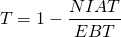
Solving T for HQN in 2018 using EBT and NIAT values from Table 5.1 we find:
(5.7)
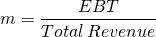
Profit margin (m) ratio
The ratio m measures the proportion of each dollar of cash receipts that is retained as profit after interest is paid but before taxes are paid.
The ratio m, is defined as:
(5.8)
In 2018, HQN had a before-tax profit margin equal to:
(5.9)
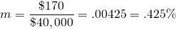
In other words, for every $1 of revenue earned by the firm, HQN earned $0.00425 in before-tax profits. Meanwhile, the after-tax profit margin m is defined as:
(5.10)
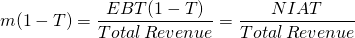
In 2018, HQN had an after-tax profit margin equal to:
(5.11)
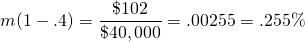
In other words, for every $1 of cash receipts, HQN earned $0.00255 in after-tax profits.
Return on assets (ROA) ratio
The ROA measures the amount of profits generated by each dollar of assets and is equal to:
(5.12)
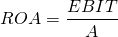
HQN’s 2018 before-tax ROA using beginning period assets is equal to:
(5.13)

Interpreted, each dollar of HQN’s assets generates $.065 cents in before-tax profits.
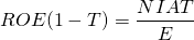
Return on equity (ROE) ratio
The ROE ratio measures the amount of profit generated by each dollar of equity after interest payments to debt capital are subtracted but before taxes are paid. Profits after interest is subtracted equals EBT (earnings before taxes). The ROE ratio can be expressed as:
(5.14)
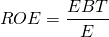
HQN’s 2018 before-tax ROE using beginning period equity is equal to:
(5.15)

After-tax return on equity, ROE(1 – T), can be expressed as EBT adjusted for taxes, or NIAT. Therefore, ROE(1 – T) can be expressed as NAIT divided by equity:
(5.16)
HQN’s 2018 after-tax ROE is equal to:
(5.17)

Interpreted, each dollar of equity generated about $0.085 in before-tax profits and $0.051 in after-tax profits during 2018.
The relationship between ROE and ROA. Before leaving profitability ratios, there is one important question: which is greater for a given firm: ROE or ROA? To answer this question, we simply define (ROE) / (E) as equal to the return assets (ROA)(A) less the cost of debt (i)(D):
(5.18)

After substituting for A, (D + E) and collecting like terms and dividing by equity E, we obtain the result in Equation \ref{5.19}:
(5.19)

Equation (5.19) reveals ROE > ROA if ROA > i; ROE = ROA if ROA = i; and ROE < ROA if ROA < i.
If ROE is not greater than ROA, then the firm is losing money on every dollar of debt. For HQN, ROE is 8.5% and greater than its ROA of 6.5%. Meanwhile HQN’s average interest rate on its debt (total interest costs divided by debt at the beginning of the period equal to i) during 2018 was equal to:
(5.20)
Efficiency Ratios
Efficiency ratios compare outputs and inputs. Efficiency ratios of outputs divided by inputs describe how many units of output each unit of input has produced. More efficient ratios indicate a unit of input is producing greater units of outputs than smaller efficiency ratios.
Consider two types of efficiency ratios: turnover (TO) ratios and turnover time (TOT) ratios. The turnover ratios measure output produced per unit of input during the accounting period, in our case 365 days. For example, suppose our TO ratio is 5. A TO ratio of 5 tells that during 365 days, every unit input produced 5 units of output.
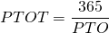
We may want to find the number of days required for a unit of input to produce a unit of output. We can answer the question by dividing 365 days by the number of turnovers that occurred during the year. This tells us the number of days required for a unit of input to produce a unit of output, what we call a turn over time, or TOT, ratio. Continuing with our example, if an input was turned into an output 5 times during the year, then dividing 365 days by 5 tells us that every turnover required (365 days)/5 = 73 days.
We now consider four TO efficiency measures: (1) the inventory turnover (ITO) ratio, (2) the asset turnover (ATO) ratio, (3) the receivable turnover (RTO) ratio, and (4) the payable turnover (PTO) ratio. We also find for each TO ratio their corresponding TOT ratio.
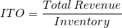
Inventory turnover (ITO) ratio
The ITO ratio measures the output (total revenue) produced by the firm’s inputs (inventory). Total revenue is a period of time measure. Inventory is a point-in-time measure. We use the beginning of the period inventory measure because it reflects the inventory on hand when revenue generating activities began. ITO is defined below.
(5.21)
The 2018 ITO ratio for HQN is:
(5.22)
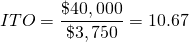
The ITO ratio indicates that for every $1 of inventory, the firm generates an estimated 10.67 dollars of revenue during the year. A small ITO ratio suggests that the firm is holding excess inventory levels given its level of total revenue. Likewise, a large ITO ratio may signal potential “stock outs” which could result in lost revenue if the firm is unable to meet the demand for its products and services.
We can find the number of days required to sell a unit of the firm’s beginning inventory, its inventory turnover time (ITOT) ratio, by dividing one year (365 days) by the firm’s ITO:
(5.23)
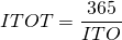
The ITOT ratio for HQN in 2018 is equal to:
(5.24)

In other words, a unit of inventory entering HQN’s inventory is sold in roughly 35 days.
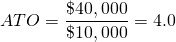
Asset turnover (ATO) ratio
The ATO ratio measures the amount of total revenue (output) for every dollar’s worth of assets (inputs) during the year. The ATO ratio measures the firm’s efficiency in using its assets to generate revenue. Like the ITO ratio, the ATO ratio reflects the firm’s pricing strategy. Companies with low profit margins tend to have high ATO ratios. Companies with high profit margins tend to have low ATO ratios.
Let A represent the value of the firm’s assets. The ATO ratio is calculated by dividing the firm’s total revenue by its total assets:
(5.25)

Using beginning of the period assets, HQN’s 2018 ATO ratio is equal to:
(5.26)
We can find the firm’s asset turnover time (ATOT) ratio, the number of days required for a dollar of assets to generate a dollar of sales, by dividing 365 by the firm’s ATO ratio. Using the ATO previously calculated for HQN in 2018 we find:
(5.27)
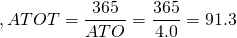
In other words, a dollar of HQN’s assets generates a dollar of cash receipts in roughly 91 days.
Receivable turnover (RTO) ratio
The RTO ratio measures the firm’s efficiency in using its accounts receivables to generate cash receipts. The RTO ratio is calculated by dividing the firm’s total revenue by its accounts receivables. Using account receivables measured at the beginning of the year, the firm’s RTO ratio measures how many dollars of revenue are generated by one dollar of accounts receivables held at the beginning of the period. The RTO reflects the firm’s credit strategy. Companies with high RTO ratios (strict customer credit policies) tend to have lower levels of total revenue than those with low RTO ratios (easy credit policies). We express the RTO ratio as:
(5.28)

Using data from HQN for 2018, cash receipts from the income statement, and accounts receivables from the ending 2017 balance sheet, we find HQN’s RTO to equal:
(5.29)

In the case of HQN during 2018, every dollar of account receivables generated $24.39 in revenue or an output to input ratio of 24.39.
We can estimate the firm’s receivable turnover time (RTOT) ratio or what is sometimes called the firm’s average collection period for accounts receivable ratio, the number of days required for a dollar of credit sales to be collected, by dividing 365 by the firm’s RTO ratio.
(5.30)
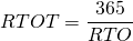
In the case of HQN during 2018, we find its RTOT ratio equal to:
(5.31)

Interpreted, it takes an average of nearly 15 days from the time of a credit sale until the payment is actually received. The RTOT ratio, like the RTO ratio, reflects the firm’s credit policy. If the RTOT is too low, the firm may have too tight of a credit policy and might be losing revenue as a result of not offering customers the opportunity to purchase on credit. On the other hand, remember that accounts receivable must be financed by either debt or equity funds. If the RTOT is too high, the firm is extending a lot of credit to other firms, and the financing cost may become excessive. Another concern is that the longer a firm extends credit, the greater is the risk that the firm’s accounts receivable will ever be repaid.
In some cases, it is useful to construct a schedule that decomposes accounts receivable into the length of time each amount has been outstanding. For example, the schedule might break the accounts receivable into: 1) the amount that is less than 30 days outstanding, 2) the amount that is 30–60 days outstanding, and 3) the amount that is more than 60 days outstanding. This breakdown provides additional information on the risk of the firm’s accounts receivable and the likelihood of repayment.
Payable turnover (PTO) ratio
The PTO ratio measures the firm’s efficiency in using its accounts payable to acquire its accrued COGS. The PTO is calculated by dividing accrued COGS (equal to cash COGS plus change in account payable) by accounts payable measured at the beginning of the year. The firm’s PTO ratio measures how many dollars of accrued COGS are generated by one dollar of accounts payable held at the beginning of the period. The PTO reflects the firm’s credit strategy. Does it prefer equity or debt financing. Firms with low PTO ratios tend to favor the use of debt to finance the firm which tends to generate higher variability in its ROE. The PTO ratio is expressed as:
(5.32)

Using data from HQN for 2018, we find its PTO to equal:
(5.33)
In the case of HQN, every dollar of accounts payable produced 9.33 dollars in accrued COGS.
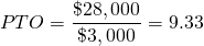
We can estimate the firm’s payable turnover time (PTOT) ratio by dividing 365 days by the firm’s PTO ratio.
The PTOT ratio measures the number of days before a firm repays its credit purchases. The PTOT formula, like the other average period ratios, is found by dividing 365 by the PTO ratio. The PTOT ratios can be expressed as:
(5.34)
HQN’s 2018 PTOT ratio is calculated as:
(5.35)

Interpreted, HQN’s PTOT ratio of nearly 39 days implies that it takes the firm an average of 39 days from the time a credit purchase is transacted until the firm actually pays for its purchase. The PTOT ratio, like the PTO ratio, reflects the firm’s credit policy. If the PTOT is too low, the firm may not be using its available credit efficiently and relying too heavily on equity financing. On the other hand, PTOT ratios that are too large may reflect a liquidity problem for the firm or poor management that depends too much on high cost short term credit.
Note of caution. Economists and others frequently warn against confusing causation and correlation between variables. Descriptive data reflected in the ratios derived in this section on efficiency ratios do not generally reflect a causal relationships between variables nor should they be used to make predictions. For example, in the previous section, we are not suggesting that PTOT can be predicted by the PTO or vice versa. The only thing that can be inferred is that PTOT times PTO will always equal 365 days.
Liquidity Ratios
A firm’s liquidity is its ability to pay short-term obligations with its current assets. Also implied by liquidity is the firm’s ability to quickly convert assets into cash without a loss in their value which would be the case if the exchange of an asset for cash required a large discount. However, before we review important liquidity ratios, we review an important liquidity measure that is not a ratio: a firm’s net working capital.
Net working capital (NWC). Even though NWC is not a ratio, it provides some useful liquidity information that should not be ignored. If NWC is positive, then CA which are expected to be converted to cash during the upcoming year will be sufficient to pay for CL, those liabilities expected to come due during the upcoming year. HQN’s net working capital, described in Table 5.2, is positive for years 2016, 2017, and 2018, suggesting the firm was capable of meeting its short-term debt obligations by using only the assets expected to be liquidated during the upcoming year.
Table 5.2. Net Working Capital for HQN
| Year | rrent CuAssets | – | Current Liabilities | = | Net Working Capital |
| 2016 | $5,910,000 | – | $5,370,000 | = | $540,000 |
| 2017 | $6,320,000 | – | $5,958,000 | = | $362,000 |
| 2018 | $7,000,000 | – | $6,600,000 | = | $400,000 |
Another aspect of HQN’s NWC is its trend. Is NWC increasing or decreasing over time? We measure the trend in NWC by calculating the change in NWC between calendar years. HQN’s NWC decreased by $178,000 during 2017 ($362,000 – $540,000). It increased by $38,000 during 2018 ($400,000 – $362,000).
The decrease in NWC during 2017 and the slight increase in 2018 calls for an explanation. Was the drop in NWC justified? Did it represent a conscious liquidity decision by the firm? Was it due to external forces? It is the duty of financial managers to find answers to these questions.
Current (CT) ratio
Liquidity ratios measure a firm’s ability to meet its short-term or current financial obligations with short-term or current assets. The CT ratio is the most common liquidity measure. It combines two point-in-time measures from the balance sheet, current assets (CA), and current liabilities (CL). The point-in-time measures of the two numbers must be the same. We write the CT ratio as:
(5.36)

In principle we would like to see the CT ratio exceed one (CT > 1), because it suggests that for every dollar of CL there is more than one dollar of CA sufficient to cover the liquidation of CL if necessary. If the CT ratio is less than one (CT < 1), then liquidating current assets will not generate enough funds to pay for the firm’s maturing current liabilities obligations which may create a significant problem. If the firm’s current liabilities exceed its current assets, the firm may have to liquidate long-term assets to meet it current obligations. But liquidating long-term (usually illiquid) assets is often costly to do because they cannot be easily converted to cash and end up being sold for a price less than their value to the firm.
The current ratio is constructed from the firm’s balance sheet (see Table 5.1). The CT ratio for HQN at the beginning of 2018 (the end of 2017) was:
(5.37)
HQN’s beginning 2018 CT ratio value of 1.06, suggests that its current liquid resources were just sufficient to meet its current obligations.
As with all the ratios we will consider, there is generally no “correct” CT ratio value. Clearly a firm’s CT ratio can be too low, in which case the firm might have difficulty paying its maturing short-term liabilities. Nevertheless, a CT < 1 does not mean that a firm will not be able to meet its maturing obligations. The firm may have access to other resources that can be used to help meet maturing obligations, such as earnings from operations, long-term assets that could be liquidated, debt which could be restructured, and/or investments in depreciating assets which can be delayed.
On the other hand, a firm’s CT ratio can be too high. CA usually earn a low rate of return and holding large levels of current assets may not be profitable to the firm. It may be more efficient to convert some of the CA to long-term assets that generate larger expected returns. To illustrate, think of the extreme case of a firm that liquidates all of its long-term assets and holds them as cash. The firm might have a large CT ratio and be very liquid, but liquid assets are unlikely to generate a high rate of return or profits.
Quick (QK) ratio
The QK ratio is sometimes called the acid-test ratio. The QK ratio is very similar to the CT ratio, except that inventories (INV), another point-in-time measure obtained from the firm’s balance sheet, are subtracted from CA. The QK ratio is defined as:
(5.38)
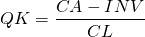
In forming the QK ratio, inventories are subtracted because inventories are most often the least liquid of the current assets, and their liquidation value is often the most uncertain. Thus the QK ratio provides a more demanding liquidity measure than the firm’s CT ratio.
Using balance sheet data from Table 5.1, we find the beginning 2018 QK ratio for HQN equal to:
(5.39)
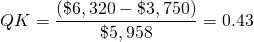
In other words, liquidating all current assets except inventory will generate enough cash to pay for only 43 percent of HQN’s current liabilities. Once again, there is no right or wrong QK ratio. This partly depends on the form of one’s inventories. Product inventories are liquid. Inventories of inputs are less liquid. Clearly, HQN’s liquidity is much lower if its inventory is not available to meet currently maturing obligations. Nevertheless, similar to the CT ratio, a QK ratio of less than one does not necessarily mean the firm will be unable to meet the maturing obligations.
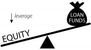
Leverage Ratios
A lever is bar used for prying or dislodging something. We can move more weight with a lever than by applying force directly. The concept of leverage has application in finance. In finance, we define leverage ratios as those ratios used to describe how a company obtains debt and assets using its equity, as a lever. There are several different leverage ratios, but the main components of leverage ratios include debt, equity, and assets. A common expression that associates leverage with equity and debt is: How much debt can we raise (leverage) with our equity?
In general, higher leverage ratios imply greater amounts of debt financing relative to equity financing and greater levels of risk. Greater levels of firm risk also imply less ability to survive financial reversals. On the other hand, higher leverage is usually associated with higher expected returns. Here, we consider two key leverage ratios: (1) debt-to-equity ratio (DE) and (2) equity multiplier ratio (EM).
Debt-to-equity (DE) ratio
 DE ratios
are the most common leverage ratios used by financial managers.
They combine two point-in-time measures from the same balance
sheet. The DE ratio measures the extent to which the firm uses its
equity as a lever to obtain loan funds. As the firm increases its
DE ratio, it also increases its control over more assets.
DE ratios
are the most common leverage ratios used by financial managers.
They combine two point-in-time measures from the same balance
sheet. The DE ratio measures the extent to which the firm uses its
equity as a lever to obtain loan funds. As the firm increases its
DE ratio, it also increases its control over more assets.
The DE ratio is equal to the firm’s total debt (D) divided by its equity (E). If dollar returns on assets exceed the dollar costs of the firm’s liabilities, having higher DE ratios (greater leverage) increases profits for the firm. We write the firm’s DE ratio as:
(5.40)

In general, having a lower DE ratio is preferred by creditors, because more equity funds are available to meet the firm’s financial obligations. (Why?) HQN’s DE ratio at the beginning of 2018 was:
(5.41)
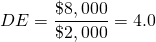
Interpreted, HQN’s DE ratio of 4 implies that each dollar of its equity has leveraged $4.00 of debt. As with liquidity ratios, there is no magic value for DE ratios. If too much debt is used per dollar of equity, the risk of being unable to meet the fixed debt obligations can become excessive. On the other hand, if too little debt is used, the firm may sacrifice returns that can be realized through leverage.
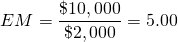
Equity multiplier (EM) ratio
 The
EM ratio is equal to the firm’s total assets A divided by its
equity E. The EM ratio tells us the number of assets leveraged by
each dollar of equity. The EM ratio like the DE ratio combines two
point-in-time measures from the balance sheet. The EM ratio is a
financial leverage ratio that evaluates a company’s use of equity
to gain control of assets.
The
EM ratio is equal to the firm’s total assets A divided by its
equity E. The EM ratio tells us the number of assets leveraged by
each dollar of equity. The EM ratio like the DE ratio combines two
point-in-time measures from the balance sheet. The EM ratio is a
financial leverage ratio that evaluates a company’s use of equity
to gain control of assets.
The EM ratio is particularly useful when decomposing the rate of return on equity using the DuPont equation that we will discuss later in this chapter. The formula for EM can be written as:
(5.42)

HQN’s assets and equity are used to calculate its EM at the beginning of 2018, and can be expressed as:
(5.43)
Leverage ratios are often combined with income statement measures to reveal important information about the riskiness of the firm beyond those provided by leverage ratios. We need to include income and cash flow data to answer the question: what is the optimal leverage ratio? We considered these issues when we earlier examined repayment capacity ratios.
Other Sets of Financial Ratios
Other sets of financial ratios besides SPELL ratios have been proposed and used elsewhere. For example, one popular set of ratios is referred to as the Sweet 16 ratios. These are compared to the SPELL ratios in Table 5.3.
Table 5.3. Comparing Sweet 16 Ratios with SPELL ratios
| SPELL Ratios | Sweet 16 List | Comments |
| (S)olvency | Solvency | Same ratios. |
| (P)rofitability | Profitability | Same ratios. |
| (E)fficiency | Efficiency | Same ratios. |
| (L)iquidity | Liquidity | Same ratios. |
| (L)everage | Repayment Capacity | Different interpretation. Equates repayment capacity with leverage. |
The DuPont Equation
The DuPont equation equals ROE multiplied by two identities assets (A) over A and total revenue over total revenue.
(5.44)

The second half of Equation \ref{5.44}, after substituting and rearranging ratios, shows that ROE depends on the asset turnover ratio (ATO), sales margin (m) and the equity multiplier (EM) ratio:
(5.45)

The DuPont equation is important because it provides a detailed picture of the firm’s ability to generate profits efficiently from its equity across several of the SPELL ratios. The first ratio measures operating efficiency using the firm’s profit margin ratio m. The second ratio measures asset use efficiency using the firm’s asset turnover ratio ATO. And the third ratio measures financial leverage or risk using the firm’s equity multiplier ratio EM.
| ROE depends on = |  |
Efficiency in generating profits from sales |  |
Efficiency in generating sales from assets | |
Amount of assets leveraged by each dollar of equity |  |
The DuPont is only one of a large number of DuPont-like equations. Multiplying by ROE assets/assets and one of the following: accounts receivables/accounts receivables, inventories/inventories, and accounts payables/accounts payables produces many versions of the DuPont equation. We list a few possibilities below:
(5.46)
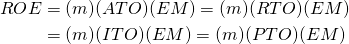
The interdependencies described in the DuPont equation help us to perform strengths and weaknesses analysis. HQN’s DuPont equation for 2018 is found using previously calculated values for m, ATO, and EM:
(5.47)

Since our ROE calculation of 8.5% equals the DuPont calculation of ROE, we are confident that our calculations, which mix point and period of time measures, are consistently calculated and reflect the interdependencies of the system. Comparing the components of the DuPont equation with industry standards we find:
| ROE depends on = | |
m: lowest quartile of the industry |  |
ATO: highest quartile of the industry | |
EM: significantly higher than the highest quartile of the industry |  |
Based on the above analysis, the ROE is at or near the industry average despite a weak profit margin because its ATO and EM are both high. HQN is efficient in its generation of cash receipts from assets and it is also highly leveraged so that as long as its average cost of debt is less than its ROA, its ROE increases.
To explore the profit margin further, note that the low profit margin is determined by EBT that in turn depends on the level of cash receipts and the cost to generate that level of cash receipts. Our earlier analysis suggested that operating costs and interest costs were relatively high, and these may be having a major impact on the profit margin.
Looking at the ATO ratio, we see that fixed assets impact the ratio, and we were concerned that the firm may not be reinvesting enough in replacing assets. Failing to replace assets as they are used up would artificially inflate the ATO and the firm’s ROE. Also, the inventory levels may be too high. Lowering the inventory levels would increase the ATO and improve ROE. Finally, the high level of leverage helped ROE but is putting the firm in a risky position. The large withdrawal of equity in 2018 has further increased this risk.
Comparing Firm Financial Ratios with Industry Standards
Financial ratios calculated for an individual firm can be made more useful by having a set of standards against which they can be compared. One might think of the limited usefulness of one’s blood pressure readings without some reference level of what is considered a normal of healthy blood pressure. Consider how one can learn more about a firm by comparing it to similar firms in the industry or by comparing it to the distribution of ratios of similar firms.
Major sources of industry and comparative ratios include: Dun and Brad- street, a publication of Dun and Bradstreet, Inc.; Robert Morris Associates, an association of loan officers; financial and investor services such as the Standard and Poor’s survey; government agencies such as the Federal Trade Commission (FTC), Securities and Exchange Commission (SEC), and Department of Commerce; trade associations; business periodicals; corporate reports; and other miscellaneous sources such as books and accounting firms. Table 5.4 shows selected HQN’s ratios for 2018, as well as ratios for other firms in the industry. The industry ratios are broken into quartiles. For example, 1/4 of the firms in the industry have current ratios above 2.0.
Table 5.4. HQN ratios for
2018 & Industry Average Ratios in Quartiles
Open HQN Coordinated Financial Statement in MS Excel
| Ratios | HQN for 2018 | Lower Quartile | Median | Upper Quartile |
| SOLVENCY RATIOS | ||||
| TIE (times interest earned) | 1.35 | 1.6 | 2.5 | 5.8 |
| DS (debt-to-service) | 1.02 | 0.9 | 1.4 | 3.3 |
| PROFITABILITY RATIOS | ||||
| m (margin) | 0.43% | 0.44% | 1.03% | 1.79% |
| ROA (return on assets) | 6.50% | 0.66% | 3.30% | 7.00% |
| ROE (return on equity) | 8.50% | 2.10% | 10.70% | 17.20% |
| EFFICIENCY RATIOS | ||||
| ITO (inventory turnover) | 10.67 | 4.8 | 7.7 | 14.9 |
| ITOT (inventory turnover time) | 34.21 | 76.04 | 47.40 | 24.50 |
| ATO (asset turnover) | 4 | 1.5 | 3.2 | 3.9 |
| ATOT (asset turnover time) | 91.25 | 243.33 | 111.06 | 93.59 |
| RTO (receivables turnover) | 24.40 | 15.21 | 11.41 | 8.90 |
| RTOT (receivables turnover time) | 14.96 | 24 | 32 | 41 |
| PTO (payable turnover) | 9.33 | 9.36 | 12.59 | 15.21 |
| PTOT (payable turnover time) | 39.12 | 39 | 29 | 24 |
| LIQUIDITY RATIOS | ||||
| CT (current) | 1.06 | 0.9 | 1.3 | 2 |
| QK (quick) | 0.43 | 0.5 | 0.7 | 1.1 |
| LEVERAGE RATIOS | ||||
| DE (debt-to-equity) | 4 | 2.8 | 1.9 | 0.9 |
| EM (equity multiplier) | 5 | 3.8 | 2.2 | 3.24 |
Using Financial Ratios to Determine the Firm’s Financial Strengths and Weaknesses
Comparing SPELL ratios with industry standards. In what follows we compare the ratios computed for HQN with the ratios calculated for similar firms. Comparing HQN’s SPELL ratios with industry standards is the essence of strengths and weaknesses analysis and answers the question: what is the financial condition of the firm?
In Table 5.4, the industry is described by the ratio for the firm, the median firm, and the average of firms in the upper and lower quartile of firms. Consider how comparing HQN to the other firms in its industry might allow us to reach some conclusions about HQN’s strengths and weaknesses and to determine its financial condition.
Solvency ratios. HQN’s solvency ratio compared to its industry indicates that it may have a difficult time paying its fixed debt obligations out of earnings. The TIE ratio in 2018 is 1.35 which is less than the industry’s lowest quartile. HQN’s DS ratio in 2018 is 0.94, which implies that only about 94 percent of the firm’s interest and principal can be paid out of current earnings which is only slightly higher than the industry’s lowest quartile. In effect, compared to industry standards, HQN’s significant weakness is its solvency. HQN will need to refinance, raise additional capital, or liquidate some assets in order to make the interest and principal payments and remain in business.
Profitability ratios. Compared to industry averages, HQN is profitable. Its ROE is reasonably close to the industry average and its ROA is close to the upper quartile industry average. Paradoxically, HQN’s m margin is close to the industry’s lowest quartile average.
Efficiency ratios. Compared to the industry averages, HQN is very efficient. Both HQN’s ITO and ATO ratios are near the top in its industry. Its ITO ratio in 2018 was 10.67, indicating that HQN has sold its inventory over 10 times during the year. This ITO ratio is above the median value for firms in this industry of 7.7, and strong. The ATO ratio has a 2018 value of 4.0, indicating the firm had sales of 4 times the value of its assets, compared to an industry median of 3.2 which is in the upper quartile of firms in its industry. The firm appears to be using assets efficiently which undoubtedly contributes to HNQ’s profitability even though its margin in low.
The RTOT ratio has a 2018 value of 14.96. This value is well below industry averages, and raises a question about the firm’s credit policies. The industry average RTOT was 32 and suggests that HQN might consider a more generous credit policy. On the other hand, HQN’s PTOT ratio is 39 and is in the lowest quartile for the industry. This suggests that HQN is depending on dealer supplied credit more than other firms in its industry because of its low solvency. Still, HQN’s strength may be its efficiency.
Liquidity ratios. The current ratio is 1.06, which suggests the firm is liquid, but barely. Its ratio is near the lower quartile of firms in the industry. The quick ratio is 0.43, suggesting the firm cannot meet its short-term obligations without relying on inventory. HQN’s quick ratio is in the lower quartile of firms in the industry, indicating that the firm is less liquid than most of its competitors and is an HQN weakness.
Leverage ratios. The leverage ratios indicate that the HQN’s use of debt is high. Comparison with industry ratios shows that HQN is highly leveraged relative to other firms in the industry. As long as ROA exceeds the average interest costs of debt, high leverage increases the firm’s profitability—but increases its risk associated with adverse earnings.
Limitations of Ratios
While ratio analysis can be a powerful and useful tool, it does suffer from a number of weaknesses. We discussed earlier how the use of different ac- counting practices for such items as depreciation can change a firm’s financial statements and, therefore, alter its financial ratios. Thus, it is important to be aware of and understand accounting practices over time and/or across firms.
Difficult problems arise when making comparisons across firms in an industry. The comparison must be made over the same time periods. In addition, firms within an “industry” often differ substantially in their structure and type of business, making industry comparisons less meaningful. Another difficulty is that a departure from the “norm” may not indicate a problem. As mentioned before, a firm might have apparent weaknesses in one area that are offset by strengths in other areas.
Furthermore, things like different production practices in a firm may require a different financial structure than other firms in the industry. Additionally, shooting for financial ratios that look like the industry average may not be very desirable. Would you want your business to be average?
Inflation can have a significant impact on a firm’s balance sheet and its corresponding financial ratios. As a results, it is important to keep in mind the difference between a capital item’s book value and it market value. Firms that keep a set of market value financial statements in addition to their book value financial statements should conduct financial analysis with both their book value and market value financial statements.
We should recognize that a single ratio does not provide adequate information to evaluate the strength or weakness of a firm. A weak ratio in one area might be offset by a strong ratio in another area. Likewise, a perfectly healthy firm, from a financial standpoint, may have some special characteristics which result in a ratio which would be out of line for other firms in the industry who do not have these characteristics.
Finally, it must be understood that financial analysis does not in itself provide a management decision. The analysis provides information which will be a valuable input into making management decisions, but there is no “cook book” formula into which you plug the financial analysis number and produce the correct management decisions.
Financial ratios can be an effective strengths and weaknesses analysis tool. Their principal use is to assess the firm’s ability to survive. To survive in the long term, the firm must be profitable and solvent. Profitability is defined as the difference between a firm’s revenues and its expenses. Solvency is the firm’s ability to meet its cash obligations when they become due. Solvency depends on the firm’s holdings of liquid assets—assets that can easily and with little expense be converted into cash in the current period.
If a firm is not both profitable and solvent, it cannot survive in the long term. In the short term, a firm can be solvent but not profitable. For a limited time, an unprofitable firm can convert assets to cash and remain solvent by borrowing, refinancing existing debt, selling inventory, liquidating capital assets, increasing accounts payable, or depleting its capital base. These acts may improve the firm’s solvency in the short run, but are likely to erode the firm’s future profitability.
In contrast, a firm may be profitable and not solvent, in which case it cannot survive even in the short term. Once a firm fails to meet its cash flow obligations, even if it is profitable, in most cases it loses control over its assets. Therefore, short-term survival may require some firms to sacrifice profitability for solvency. Thus, financial managers must monitor both the firm’s solvency and profitability. An appropriately constructed set of financial ratios will allow financial managers to monitor both the firm’s profitability and solvency.
Financial ratios may also provide information about the liquidity of the firm, which is related to the firm’s solvency because the firm’s liquidity position tells us something about the firm’s ability to meet unforeseen outcomes and survive. Also related to the firm’s solvency and liquidity is the probability of achieving different rates of return. Measures of the probability of alternative rates of return are sometimes examined under the general heading of risk, a subject we will return to later in this book (see Chapter 15).
Strengths and Weaknesses Summary
How do we summarize our strengths and weaknesses analysis? One way is to assign a grade to each of the SPELL categories ranging from 5 (superior) to 1 (on life support). Clearly, the grades assigned are somewhat subjective, but perhaps useful, in summarizing a great deal of financial information. Then what? Do we assign equal weight to each of the SPELL categories depending on their relative importance? The answer to this question depends on the vision, goals, and objectives of the firm manager. To complete this discussion of how to assign weights to the SPELL categories, we treat them equally important in this example—although a strong case exists for assigning a greater weight to profitability measures. In Table 5.5 we summarize our strengths and weaknesses ratings.
Table 5.5. Summary of HQN’s 2018 Financial Strengths & Weaknesses
| SPELL Category | weights | Grades: 5 (very strong) to 1 (very weak) |
| Solvency | .2 | 2.0 |
| Profitability | .2 | 3.0 |
| Efficiency | .2 | 4.0 |
| Liquidity | .2 | 3.0 |
| Leverage | .2 | 2.0 |
| Weighted Summary | 2.8 |
Summary and Conclusions
When using financial ratios from one’s own firm and comparing them with industry standard ratios, it is often useful to take notes or summarize the major points as you work through the ratio analysis. In our analysis of HQN, the firm is highly leveraged and is in a risky position. We might ask why is the firm relying so heavily on debt and why is its equity being withdrawn at such a relatively high rate? The overhead expenses seem to be too high. Why? How can the situation be improved? Why are the firm’s assets being depleted? What is the cause of the increasingly high level of inventory being held?
After gathering information on these questions and others, the firm’s financial manager may produce a detailed strengths and weaknesses report. In the report, key financial management issues can be explored, and forecasts of future financial needs and situations can be made. Continued monitoring of the firm’s financial statements and ratios will allow the firm’s management to gain solid understanding of the relationship between the firm’s operations and its financial performance and to recommend changes when required.
Questions
When calculating 2018 ratios, please refer to Tables 4.1, 4.4A or 4.4B, and 4.6 in Chapter 4. When asked for industry standard comparisons, use industry measures provided in Table 5.4.
- Explain why financial statement data is made more useful by forming SPELL ratios?
- Describe the kinds of questions related to the firm’s financial strengths and weaknesses each of the SPELL ratios can help answer.
- Calculate the 2018 SPELL ratios for Friendly Fruit Farm (FFF) described in Chapter 4.
- Do FFF’s DS and TIE ratios, both solvency ratios, tell consistent stories? Defend your answer.
- Explain why a firm might be reluctant to meet its short-term liquidity needs by liquidating long-term assets.
- Describe the connections between the m ratio and FFF’s ROE.
- What is the essential difference between ROA and ROE profit measures? What do they each measure?
- What conditions guarantee that ROE > ROA or that ROA > ROE?
- Explain the connections between efficiency and ROE or ROA measures.
- Create an efficiency ratio for your class preparation efforts? (Hint: what are the inputs and what are the outputs?) What could you do to improve the efficiency of your class preparation efforts?
- What might be implied by very high or very low ITO ratios?
- Calculate ITO ratios using 2018 total revenue measures for FFF. Then compare your results with ITO ratios using accrued COGS. Explain the differences.
- The optimum RTOT ratio seeks to balance the need to generate cash receipts by offering easy credit versus the need to meet liquidity need by limiting its accounts receivable. Looking at the financial statements for HQN, what is an ideal RTOT ratio (state a number)? Defend your ideal number RTOT number, and if it is different than HQN’s actual number, what actions could you take to align HQN’s actual RTOT to its ideal RTOT?
- Explain why it is difficult to compare net working capital numbers between firms.
- The DuPont equation allows us to decompose the ROE measure. Replace total revenue with COGS in Equation \ref{5.45} and recalculate the components of the revised DuPont equation. Interpret the results. Does the resulting equation still equal HQN’s ROE?
- Calculate and compare FFF CT ratios at the end of years 2017 and 2018. What can you learn from the changes in FFF’s CT ratios? Compare FFF CT ratios with industry standards. What do you learn from the comparison?
- Using FFF’s QK ratios at the end of years 2017 and 2018, what strengths and weaknesses score would you assign to its liquidity?
- Suppose FFF’s long-term debt was 10% above the book value of their long-term assets and only 50% of the current value of their long-term assets. Calculate DE ratios using current and book values of their long-term assets. If FFF were applying for a loan, which DE ratios would they most likely present?
- If ROA exceeds the average costs of the firm’s liabilities, having higher DE ratios (greater leverage) increases profits for the firm. Why might lenders want lower DE ratios while borrowers may want higher DE ratios?
- Compare firms with low ITO ratios such as jewelry stores with firms with high ITO ratios like grocery stores or gas stations. How might their profit margin requirements for success differ? Explain.
- Using FFF’s SPELL ratios and the industry standards used to evaluate HQN’s strengths and weaknesses, write a brief report of FFF’s financial strengths and weaknesses. Organize your report into the five SPELL categories: solvency, profitability, efficiency, liquidity, and leverage. Complete a table similar to Table 5.5 that was prepared for HQN. What is the summary measure of FFF’s financial strengths and weaknesses?