19: Financial Investments
- Page ID
- 12764

After completing this chapter, you should be able to: (1) distinguish between financial investments and capital investments; (2) recognize the different kinds of financial investments; and (3) evaluate the different kinds of financial investments using present value (PV) models developed in earlier chapters.
To achieve your learning goals, you should complete the following objectives:
- Distinguish between financial investments and nonfinancial investments.
- Learn how PV tools can be used to analyze financial investments using methods similar to those used when comparing nonfinancial investments.
- Learn to distinguish between financial and nonfinancial objectives.
- Learn the role of brokers, dealers, and financial intermediaries in the securities markets.
- Learn how to value riskless securities such as time deposits.
- Learn why Albert Einstein called compounding interest “the greatest mathematical discovery of all time”.
- Learn the nature of bonds and the variables that determine their value.
- Learn how tax rates affect the value of financial investments.
Introduction
In its broadest meaning, to invest means to give up something in the present for something of greater value in the future. Investments, what we invest in, can differ greatly. They may range from lottery tickets and burial plots to municipal bonds and corporate stocks. It is helpful to organize these investments into two general categories: real and financial. Capital, or real, investments involve the exchange of money for nonfinancial investments that produce services such as storage services from buildings, pulling services from tractors, and growing services from land. Financial investments involve the exchange of money in the present for a future money payment. Financial investments include time deposits, bonds, and stocks.
This chapter applies PV models developed earlier to financial investments. Large corporations and other business organizations require financial investments from a large number of small investors to provide funds for operation and growth. The collection of these funds would be impossible if each investor were required to exercise a managerial role over them. Moreover, the collection of investment funds from a large number of small investors would be impossible unless the investors could be assured of investment safety and limited liability. A number of financial investments have been designed to overcome these and other investment obstacles.
The market in which financial investments are traded is called the securities market or financial market. Activities in the financial markets are facilitated by brokers, dealers, and financial intermediaries. A broker acts as an agent for investors in the securities markets. The securities broker brings two parties together to obtain the best possible terms for his or her client and is compensated by a commission. A dealer, in contrast to a broker, buys and sells securities for his or her own account. Thus, a dealer also becomes an investor. Similarly, financial intermediaries (e.g. banks, investment firms, and insurance companies) play important roles in the flow of funds from savers to ultimate investors. The intermediary acquires ownership of funds loaned or invested by savers, modifies the risk and liquidity of these funds, and then either loans the funds to individual borrowers or invests in various types of financial assets.
Numerous books discuss the institutional arrangements associated with securities trading. In this chapter, the focus in not on the details of trading in the securities market but on how to value financial investments or securities.
Valuation of Riskless Securities
The prices of financial investments, like other prices, are determined in markets—financial markets. The characteristics of financial markets, however, may differ significantly depending on the type of financial investment traded. Common to all financial markets, though, is that prices are established by matching the desires of buyers and sellers. Moreover, in equilibrium there is neither excess demand nor excess supply. However, equilibrium does not mean that all prospective buyers and sellers agree that an investment’s price is equal to its value. It only means that a price has been found that, in a sense, balances the different goals of buyers and sellers.
Time deposits. Time deposits are money deposited at a banking institution for a specified period of time. The main difference between different kinds of time deposits is their liquidity. Generally speaking, the less liquid the time deposits are, the greater their yield is.
The most liquid form of time deposits are sometimes known as “on call” deposits. On call deposits can be withdrawn at any time and without any notice or penalty. Examples of on call deposits include money deposited in a savings or checking account in a bank. Another kind of time deposit is a certificate of deposit (CDs). When CDs mature, they can be withdrawn or they can be held for another term. CDs are generally considered to be liquid because they are negotiable and can be re-discounted when the holder needs some liquidity.
Some time deposits must be held until maturity or suffer penalties for early withdrawal. The rate of return for these time deposits is higher than on call deposits because the requirement that the deposits be held for a designated term gives the bank the ability to invest in financial products that earn greater returns. In addition, the return on time deposits is generally lower than the average return on long-term investments in riskier products like stocks and some bonds. Some banks offer market-linked time deposit accounts which offer potentially higher returns while guaranteeing principal.
Investments in time deposits may consist of a one-time investment or a series of deposits. What all time deposits have in common is that the payment(s) is compounded until some ending date at which time they are partially or totally withdrawn. Thus, our interest is not in the present value of the payments but in their future value. The market determined price in the case of financial investments is the compound rate at which time deposits earn interest. Typically, the compound rate of interest earned on time deposits is low—partly because they provide nearly perfect liquidity—especially for time deposits for which there is no penalty nor transaction cost associated with withdrawal of funds.
Ordinary annuities and annuities due. Previously we described an annuity as a time series of constant payments made or received at the end of each period. Annuities paid and received at the end of a period are referred to as ordinary annuities. Annuities paid (or received) at the beginning of each period are referred to as annuity due payments.
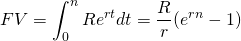
To illustrate an annuity due, consider a series of deposits R made every period, the first one occurring in the present. We write the future value Vn of the time series of deposits R compounded at rate r̂ for withdrawal in period n as:
(19.1)

Note that the first time deposit R is compounded for n periods—and is equal in value to its compounded value at the beginning of period n. Similarly, the second payment is compounded for n – 1 period and is equal to its compounded value at the beginning of period n. Finally, the last payment is made at the beginning of period n – 1 and is compounded once to find its compounded value at the beginning of period n.
To illustrate, suppose a saver deposits a $90 payment (PMT) at the beginning of each period for n = 10 periods. If the deposits are compounded at a rate of r = 2%, what amount is available for withdrawal at the beginning of period 10? We solve this problem using Excel in Table 19.1. Note that to indicate annuity due payments at the beginning of the period, “type” in the Excel future value FV function is changed from its default of zero to 1. In place of PV in the equation, we enter a blank closed with a comma.
Table 19.1. The Future Value
of 10 Annuity Payments of $90 Compounded at 2%
Open Table 19.1 in Microsoft Excel
| B6 | Function: | =FV(B4,B5,B3,,B2) | |
| A | B | C | |
| 1 | The Future Value of 10 Annuity Due Payments of $90 Compounded at 2% | ||
| 2 | type | 1 | |
| 3 | PMT | ($90.00) | |
| 4 | rate | 0.02 | |
| 5 | n | 10 | |
| 6 | FV | $1,005.18 | “=FV(rate,nper,pmt,[pv],type) |
| 7 | PV | 0 | |
What our calculations determine is that at the beginning of the 10th period, we have $1,005.18 available. However, there are several other interesting questions that we might answer using our Excel formulas. For example, we might want to know how many periods would be required to have $2,000 available at some future date. Continuing with the entries already made in Excel, we add the following:
Table 19.2. Finding the
Number of Annuity Due Payments Required to Earn a Future Value of
$2,000
Open Table 19.2 in Microsoft Excel
| B5 | Function: | =NPER(B4,B3,B6,B2) | |
| A | B | C | |
| 1 | Number of Annual $90 Annuity Due Payments Compounded at 2% Required to Earn a FV of $2,000 | ||
| 2 | type | 1 | |
| 3 | PMT | ($90.00) | |
| 4 | rate | 0.02 | |
| 5 | n | 29.69347722 | “=NPER(rate,pmt,FV,type) |
| 6 | FV | $2,000 | |
| 7 | PV | 0 | |
We might be interested in knowing the periodic investment required to have $2,000 available in 10 years if the investments were compounded at 2%. The required Excel formula is represented in Table 19.3.
Table 19.3. Finding the
Annuity Due Payment Required to Earn a Future Value of $2,000 in 10
Years
Open Table 19.3 in Microsoft Excel
| B3 | Function: | =PMT(B4,B5,B7,B6,B2) | |
| A | B | C | |
| 1 | Annual Annuity Due Payment Compounded at 2% Required to Earn a FV of $2,000 in 10 years. | ||
| 2 | type | 1 | |
| 3 | PMT | ($179.07) | “=PMT(rate,nper,PV,FV,type) |
| 4 | rate | 0.02 | |
| 5 | n | 10 | |
| 6 | FV | $2,000 | |
| 7 | PV | 0 | |
To reach one’s savings goal of $2,000 in 10 years at a compound rate of 2% would require a periodic payment into a time deposit at the beginning of each period equal to $179.07.
Compound Interest
The magic of compounding. It is claimed that Albert Einstein called compound interest “the greatest mathematical discovery of all time”. It is probable that no other concept in finance has more importance for investors than what is sometimes called the “wonder of compound interest.” Compounding interest creates earnings not only on the original amount saved or invested but also creates earning on the interest on earnings, and it does so period after period. Another way to describe this process is to say that compounding interest generates earnings on the investment and reinvested earnings from the investment. To realize the power of compound interest requires two things: the re-investment of earnings and time.
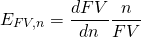
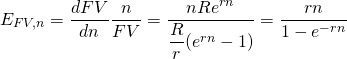
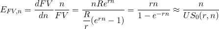
Our previous calculations confirm the importance of compound interest. In 10 payments of $90 we accumulated a future value of $1,005.18. By making an additional 8.57 payments, we doubled our future value. We found a similar effect when we increased loan payments and observed significant decreases in term. When finding the effect of increased loan payments on loan terms, we calculated the elasticity of the term of the loan with respect to the size of the loan payment. Similarly, we can find the impact of an increase in the term of periodic savings on future values (FV). We refer to this elasticity as the FV elasticity with respect to term. The derivation of the FV elasticity with respect to term is found in Derivation 19.1 at the end of this chapter. The discrete approximation to the FV elasticity with respect to n is:
(19.2)
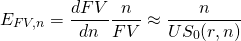
Table 19.4 provides elasticity estimates for alternative reinvestment rates and terms.
Table 19.4. Tabled Values of elasticity EFV,n = n/US0(r,n)
| n | r = .01 | r = .03 | r = .05 | r = .08 | r = .10 | r = .15 |
| 1 | 1.00% | 1.03% | 1.05% | 1.08% | 1.10% | 1.15% |
| 3 | 1.02% | 1.06% | 1.10% | 1.16% | 1.21% | 1.31% |
| 5 | 1.03% | 1.09% | 1.15% | 1.25% | 1.32% | 1.49% |
| 10 | 1.05% | 1.17% | 1.30% | 1.49% | 1.63% | 1.99% |
| 20 | 1.08% | 1.34% | 1.60% | 2.04% | 2.35% | 3.20% |
| 30 | 1.16% | 1.53% | 1.95% | 2.66% | 3.18% | 4.57% |
| 60 | 1.34% | 2.17% | 3.17% | 4.85% | 6.02% | 9.00% |
A related question with a more intuitive answer is how long does it take to double, triple, or quadruple one’s investment? The derivation for the equation that answers this question can be found in Derivation 19.2 at the end of this chapter.
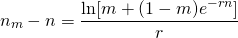
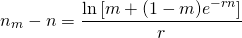
Let m be the number of times one wants to multiply his or her FV obtained at period n. Let nm equal the period in which the last deposit is made. Then we can find the number of periods (nm – n) required to increase the original FV by m times. The formula found in Derivation 19.2 is provided below:
(19.3)
To illustrate, let r = .1, n = 5, and m = 2. The number of periods required to double the FV of one’s original investment equals:
(19.4)
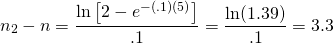
In this example, an investment consisting of 5 equal payment compounded at 10% could be doubled in additional 3.3 payments. And the investment could be tripled in:
(19.5)
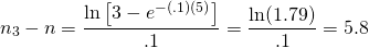
The second example illustrates the power of compounding interest. Starting after 5 periods of investing, in 3.3 more periods the FV of the investment doubled and in 5.8 additional periods the FV of the original investment tripled.
Finally, we conclude this section by constructing Table 19.5 demonstrating the power of compounding interest. The cells of the table indicate the time required to double, triple, and quadruple an initial investment for reinvestment rates of 1%, 3%, 5%, and 10%.
Table 19.5. Periods required to double, triple, or quadruple the FV of an investment consisting of 5 equal payments assuming alternative reinvestment rates.
| Alternative re-investment rates | Number of time periods required to increase the FV of the original investment m times | ||
| m = 2 (double the original FV) | m = 3 (triple the original FV) | m = 4 (quadruple the original FV) | |
| 1% | 4.8 | 9.3 | 13.7 |
| 3% | 4.4 | 8.2 | 11.6 |
| 5% | 4.0 | 7.3 | 10.2 |
| 10% | 3.3 | 5.8 | 7.8 |
The rule of 72 approximates the amount of time it takes to double your investment at a given rate of return. To apply the rule, you divide the rate of return by 72. For example, assume you invest $1000 at an interest rate of 5%. It would take 14.4 years (72/5) to double your investment to $2000.
Bonds
A bond is a financial asset frequently traded in financial markets. Bonds represent debt claims on the assets and income of the entity issuing the bond. A bond’s value is equal to the present value of its future cash flow (interest and principal) discounted at an appropriate interest rate. Bonds usually have a known maturity date at which time the bond holder receives the bond’s face or par value. Bonds are unique because their redemption or liquidation value is fixed. Typical redemption amounts are $1,000 or $10,000.
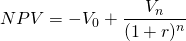
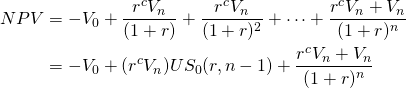
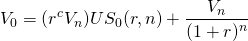
Consider the following example. Suppose a bond can be purchased at a price of V0 (an initial cash outflow) and redeemed n periods later at a cash value of Vn, a cash inflow to the bond holder. Moreover, suppose that the bond generates no cash return except when it is sold. Further, assume that the before-tax discount rate is r percent. Ignoring any tax consequences, the NPV of this bond is the sum of the cash outflow plus the present value of the cash inflow.
(19.6)
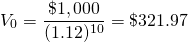
Those who purchase bonds may want to calculate the “yield” on a bond, which is the discount rate that equates the present value of the bond’s cash flow to its present market value—the bond’s internal rate of return (IRR). If, for example, the bond’s market value is $321.97 and its cash flow of $1,000 occurs at the end of year 10, then the bond’s yield, or its IRR, is 12 percent.
(19.7)
Now consider the effect of taxes. First, assume capital gains taxes are paid by the bond purchaser at rate Tg and income taxes are paid at rate T. The after-tax NPV of the bond is calculated by adjusting the discount rate to its after-tax equivalent and by subtracting from the liquidation value of the bond, the capital gains tax:
(19.8)
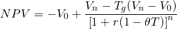
where  is the tax adjustment coefficient defined in Chapter 11. If the NPV
in Equation \ref{19.5} is zero then
is the tax adjustment coefficient defined in Chapter 11. If the NPV
in Equation \ref{19.5} is zero then  is the bond’s after-tax IRR. To find the effective tax rate we set
NPV equal to zero in equations (19.8) and (19.6) so that before-tax
cash flow discounted by the before-tax IRR in Equation \ref{19.6}
is equal to the after-tax cash flow discounted by the after-tax IRR
in Equation \ref{19.8}. Then we solve for
that makes the two equations equal. The result is:
is the bond’s after-tax IRR. To find the effective tax rate we set
NPV equal to zero in equations (19.8) and (19.6) so that before-tax
cash flow discounted by the before-tax IRR in Equation \ref{19.6}
is equal to the after-tax cash flow discounted by the after-tax IRR
in Equation \ref{19.8}. Then we solve for
that makes the two equations equal. The result is:
(19.9)

To illustrate using the numbers from our previous
example, let the before-tax IRR equal 12%, let
V0 equal $321.97, let Vn
equal $1,000, and let the income tax and the capital gains tax
T and Tg both equal 15 percent. Next
making the appropriate substitutions into Equation \ref{19.6} we
find
equal to:
(19.10)

For  the effective tax rate is reduced from 0.15 to (.66)(0.15) =
0.10.
the effective tax rate is reduced from 0.15 to (.66)(0.15) =
0.10.
In the example, just completed, we were able to
deduce a closed form solution for .
In most cases, closed form solutions are very difficult to obtain.
Nevertheless, in most practical cases involving numerical
estimates, we can still find estimates for the effective tax rate
and after-tax IRRs. We will demonstrate the empirical approach to
finding effective tax rates in the next section.
Coupons and Bonds
Most bonds, in addition to capital gains (or losses), provide “coupon” (interest) payments. The number and amount of the coupon payments will alter the NPV as well as the price of the bond. Usually, the coupon rate rc is a percentage of the redemption value of the bond.
The before-tax NPV of a bond with n coupon payments is:
(19.11)
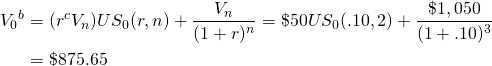
To illustrate, suppose an investor wants to find
the maximum bid price  for a three-year $1,000 bond if it offers coupon payments of
rcVn = (.05)(1,000) = $50, and
r = 10%. Then using Equation \ref{19.11} and setting NPV
equal to zero, find the maximum bid price
equal to:
for a three-year $1,000 bond if it offers coupon payments of
rcVn = (.05)(1,000) = $50, and
r = 10%. Then using Equation \ref{19.11} and setting NPV
equal to zero, find the maximum bid price
equal to:
(19.12)
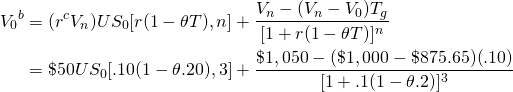
Taxes, of course, affect the NPV of bonds with coupon payments. Only now, taxes may or may not be paid on the coupon payments and capital gains. For example, coupon payments of many municipal bonds are not taxed but their capital gains are taxed. Tax exemptions, of course, raise the maximum bid price and NPVs of the bonds for all investors but especially for higher tax bracket investors. The after-tax present value of the bond with tax-exempt coupon payments is written as:
(19.13)

To illustrate, suppose an investor wants to find
the maximum bid price
for a three-year $1,000 bond if it offers coupon payments of
rcVn = (.05)(1,000) = $50 and
r = 10% and pays capital gains and income taxes at the
rate of 10%. Then using Equation \ref{19.13} and setting NPV equal
to zero, we find the maximum bid price
for the bond whose earlier maximum bid price was calculated equal
to $875.65:
(19.14)
In the application of Equation \ref{19.13}, the
discount rate was the IRR—because it was the discount rate that
resulted in NPV equal to zero. We introduced taxes into the cash
flow, but we don’t know the effective after-tax discount rate that
would set NPV equal to zero. We have to solve for
that will adjust the discount rate for taxes in the same magnitude
as were the cash flow adjusted for taxes. For Equation \ref{19.13},
we find the after-tax IRR using Excel:
Table 19.6. Finding the
After-tax IRR
Open Table 19.6 in Microsoft Excel
| B6 | Function: | =IRR(B2:B5) | |
| A | B | C | |
| 1 | Finding the After-tax IRR | ||
| 2 | Bond’s max bid price | -875.65 | |
| 3 | first coupon payment | 50 | |
| 4 | second coupon payment | 50 | |
| 5 | Salvage value (1000) + coupon payment | 1037.6 | |
| 6 | IRR | 9.59% | “=IRR(B2:B5) |
The IRR calculation of 9.59% equals the after-tax
IRR of 9.59% compared to the before tax IRR of 10%. We can find
and the effective tax rate by setting
(19.15)

From the above equation we find
= .41. Thus the effective tax rate is (.2) (.41) = 8%—far less than
the actual income tax rate of 20%.
To review the process, we began by solving for
the maximum bid price of the bond. This required that the stated
discount rate was the before-tax IRR for the bond. Then we reasoned
as follows. If the maximum bid price is the same whether calculated
on a before-tax or after-tax basis, then the effect of taxes on the
cash flow—in this case the capital gains tax—must have the same
effect on the discount rate. Thus, we required that the maximum bid
price in the after-tax model be the same maximum bid determined in
the before-tax model and solved for the after-tax IRR and the tax
adjustment coefficient
.
Common Stocks
In contrast to bonds, common stocks have neither a fixed return nor a fixed cost. The terminal value of bonds is usually fixed, but the terminal value of stocks depends on the market value of the stock at the time of sale. The equity capital generated by the sale of stock is an alternative to debt capital generated by the sale of bonds. It also is a means of sharing risk among numerous investors.
Stocks offer significant benefits for stockholders as well as the companies issuing the stocks. Stockholders have the opportunity for ownership in the major businesses of the world with the consequent share in profits while their liability is limited to their investments. Moreover, stock ownership frees them from decision-making responsibilities in the management of the company, although common stock allows its owners to vote for directors and sometimes other matters of significance facing the company.
Stock owners receive dividend payments on their stocks, usually on a quarterly basis. The amount of dividends paid on stocks is determined by a corporation’s board of directors. The board of directors’ dividend policies may influence the kinds of stock they issue and the kinds of investors they attract.
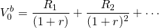
The relevant question for a potential stock purchaser is what is the maximum bid price for a particular stock? If r is the nominal discount rate, and R1, R2, ⋯ are projected dividends paid on the stock in periods 1, 2, ⋯, the maximum bid price for the stock is:
(19.16)
The model above assumes an infinite life. This assumption is consistent with the “life of the investment” principle discussed in Chapter 8 because to know the terminal value of the stock, Vn, we must know the value of the dividends in periods (n + 1), (n + 2), ⋯. Knowing all future dividends converts the problem to one in which the number of periods equals the life of the firm.
A simplified form of Equation \ref{19.16} is possible if expected dividends R1, R2, ⋯ are replaced by their expected annuity equivalent R. Then we can write:
(19.17)
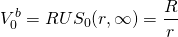
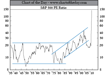
And r, the stock’s IRR, is R/V0. Thus, with long-term constant dividends of $100 and the stock valued at $1000, the rate of return is 10%. Another important ratio derived from Equation \ref{19.16} is what is commonly referred to as the price-to-earnings ratio, V0 / R = 1 / r which is often viewed as the bellwether of financial irregularities in the financial market. Higher than usual price-to-earnings ratios may signal what has been called “irrational exuberance” for the investment. Lower than usual price-to-earnings ratios may signal that the investment is undervalued.
Finally, debt capital must be repaid regardless of the financial fortunes of the business. However, the return to stockholders depends critically on the performance of the company. This makes NPV analysis of stock investments subject to considerable uncertainty.
Figure 19.1. S&P 500 PE ratio peaks at record highs.
Summary and Conclusions
This chapter has introduced concepts related to financial investments which involve exchanges of money over time. In relation to financial investments, the focus is on the amount of one’s investment available at some future period of time. We find the FV of a financial investment by compounding interest. As we demonstrated in Table 19.1, the power of compounding is truly amazing. Therefore, the advice for most investors is to invest early and continuously, and then let one’s investment grow.
Time deposits represent an important financial investment opportunity. These differ mostly in their liquidity—those that are least liquid are also the ones with the higher yields. Bonds are an important class of financial investment. In contrast to most other financial investments, their liquidation value is fixed. What is not fixed is their purchase price which is established in the market and depends on their yield—their expected IRR.
One of the interesting aspects of bonds is the way they are taxed. Often when bonds are issued by municipalities and some other institutions, they receive special tax considerations. In the extreme neither their coupon payments nor their capital gains are taxed. In other circumstances, capital gains are taxed and coupon payments are not. Regardless, an important question is how do special tax provisions provided with some bonds affect their after-tax IRRs. While the effective after-tax IRR can sometimes be found in a formulaic expression, often they are too complicated to be expressed in a closed form solution but can be found numerically by calculating the before and after-tax IRRs.
Finally, we only introduced the concept of common stocks. Investments in common stocks are most often discussed in the context or risk analysis and include discussions of many alternative of risk response strategies. A more complete discussion of investments in stocks is beyond the scope of this financial management text.
Questions
- To invest means to give up something in the present for something of value in the future. Can you describe three of your most important personal investments? Describe what you sacrificed including money and time, and describe your expected future returns.
- Describe the difference between real and financial investments. Also describe how the investment settings for real and financial investments may differ.
- Describe the main characteristics of alternative types of time deposits? What are the rates of return currently offered by major banks or credit unions on alternative types of time deposits?
- Suppose a saver invests $65 in a time deposit at the beginning of each period for 10 periods. If the deposits are compounded at a rate of 4%, what amount is available for withdrawal at the beginning of period 11?
- Suppose a young couple now renting an apartment wants to invest in their own home. The average price range of their desired home is approximately $250,000. If they make monthly deposits in a time deposit account at the beginning of the period for 5 years and their deposits earn an APR compound rate of 3%, what would be the required size of their monthly deposit to pay for the 20% required down payment of the price of their home ($50,000)? If they desired to save the required down payment in three years, what would be the required size of their monthly deposits?
- It is claimed that Albert Einstein called compound interest “the greatest mathematical discovery of all time.” What is it about compounding that is so important that he would make such a claim? Do you agree? If so, why? If you disagree, what would be an alternative mathematical discovery of greater importance?
- Describe in words the meaning of the elasticity of the future value of an investment with respect to its term. Then calculate the elasticity of the future value of an investment compounded at an APR rate of 4% for 12 periods. How would the elasticity measure change if the compound rate were increased to 7%? Can you explain the direction of the change?
- Find the number of periods required to double the future value of an investment compounded for 5 periods at alternative reinvestment rates of 2%, 4%, and 8%.
- An investor desires to save $10,000. If the compound rate is 3% per month and the investor plans on saving $200 at the beginning of each month, how many months will be required for the investor to reach her savings goal of $10,000? Once the saving goal is reached, how many addition months will be required for the saver to double the amount saved if she saves at the same rate?
- Consider an 8-year bond with a par value of $10,000. If the purchase price of the bond is $4,250, what is the yield on the bond? (Ignore the influence of taxes.)
- What is the relationship between the bond’s yield (its IRR) and the bond’s purchase price? What would you expect to happen to the bond’s purchase price if the expected yield on the bond increased? Please explain.
- In the example illustrating Equation \ref{19.8}, the effective tax rate for a bond purchaser was found to equal θT = .66(.15) = 10%. Please recalculate the effective tax rate in the example assuming the capital gains tax rate is only 50% of the income tax rate. In other words, if the capital gains tax rate is 7.5%, what is the bond purchaser’s effective tax rate? How does lowering the effective tax rate change the firm’s effective after-tax IRR?
- Consider the equation:
(Q19.1)

where
is the after-tax IRR of a bond.
Next consider the equation:
(Q19.2)
where r is the before-tax IRR of the bond.
Then assume that
V0 = $500, Vn = $1000,
rcVn = .04($1,000) = $40, T
= 20%, and Tg = 10%. Find the before-tax and
after-tax IRRs using the two equations described in this question
and the values listed. Then use the before-tax and after- tax IRRs
to find the value of the tax-adjustment coefficient .
- Compare the rule of 72 with the actual time required to double your investment.
Derivation 19.1.
The derivation of the elasticity of future value (FV) with respect to term:
The elasticity of FV with respect to n is defined as:
(19.i)
The future value of n payments compounded at rate r is equal to:
(19.ii)
And the derivative of FV with respect to n is:
(19.iii)

Substituting into the elasticity formula we find:
(19.iv)
The discrete approximation of the elasticity of FV with respect to n is:
(19.v)
Derivation 19.2.
Deriving the formula for calculating the number of periods to double the FV of an n period investment reinvested at an interest rate of r%.
To begin, the future value (FV) of an n period investment R compounded at rate r is equal to:
(19.vi)

Now m times the FV of the original investment is set equal to the same investment compounded for nm periods:
(19.vii)

and simplifying by equating the two integrated equations above we find:
(19.viii)

Then solving for the difference between (nm– n), we find the time it takes to increase the FV of the original investment at period n by m times.
(19.ix)