
15: Homogeneous Risk Measures
- Page ID
- 12760

After completing this chapter, you should be able to: (1) define and measure risk; (2) understand how a person’s risk aversion affects his/her resource allocation; (3) distinguish between direct and indirect outcome variables; and (4) evaluate alternative risk response strategies available to financial managers including sharing risky outcomes, purchasing insurance, diversifying investments, purchasing risk reducing investments, and choosing an optimal capital structure.
To achieve your learning goals, you should complete the following objectives:
- Learn how to describe risky events by assigning a random variable to their outcomes and by assigning a probability density function (pdf) to the random variable.
- Learn how measure the variability and central tendencies of random variables using the expected values and variances of their probability density functions.
- Learn how risk premiums can be used to measure the cost of risk.
- Learn how to describe the risky choice set facing firm managers using expected value-variance (EV) efficient sets.
- Learn about the normal probability density function and understand why it is so important when describing risky events.
- Learn how sharing risk with others can be a useful response to risk.
- Learn how purchasing insurance can be a useful response to risk.
- Learn how diversification can be a useful response to risk.
- Learn how purchasing risk-reducing inputs can be a useful response to risk.
- Learn how leverage affects the level of risk facing the firm.
Introduction
The adjective “uncertain” describes an event (such as a hurricane or a football game) whose outcomes are not known with certainty. An uncertain event must have at least two possible outcomes, and it usually has more. In an earlier time, a distinction was made between risky events and uncertain events based on the information available for identifying an event’s possible outcomes and predicting the probabilities of those outcomes. For example, the flip of a coin is a familiar event with two outcomes: heads (H) and tails (T). Based on past trials or logic, we can infer that the probability of a heads (tails) appearing when a fair coin is tossed is about 50 percent. Some may call this event risky because we have good information about the possible outcomes and the probability of their occurrence.
Now consider a different event: the toss of a thumbtack.[1] What is the probability that the thumbtack will land on its side versus landing on its head? Because we are not familiar with this event and cannot assign probabilities to its outcomes based on our past experience or logic, this event might be called uncertain.
For many, the distinction between risky events and uncertain events is no longer important, and most researchers assign the adjectives uncertain and risky to events interchangeably. One reason many do not distinguish between risky and uncertain events is because the assignment of probabilities to event outcomes is subjective (we never have enough information to be absolutely certain about either possible outcomes or their probabilities) and may be based on other factors besides logic and past observations including hunches, omens, experiences of others in irrelevant circumstances, and advice from unqualified persons to name a few.
A distinction between risky and uncertain events may still be useful. People appear to refer to events as uncertain when the event’s outcomes are not known with certainty. It also appears popular to refer to uncertain events as risky when they are uncertain and their occurrence alters the decision maker’s well-being. Thus, only risky events matter, regardless of one’s confidence in the probabilities of various outcomes (e.g. the toss of a coin versus the toss of a thumbtack).
The study of risky events, of course, has application to capital budgeting problems. When we estimate future cash flow used in analyzing capital budgeting decisions, we are estimating risky outcomes associated with a risky event. Thus, we are faced with the challenge of satisfying the homogeneous measures principle applied to risk by adjusting future cash flow projections of a challenger and the cash flow predictions used to find the IRR of the defender to their certainty equivalent value that we will define in this chapter.
Statistical Concepts Useful in Describing Risky Events and Risky Outcomes
Probability density function. A probability density function (pdf) is a function that assigns probabilities to outcomes of risky events. For example, the toss of a fair coin is an event with outcomes showing a heads (H) or a tails (T). The pdf for this event may assign to H the probability of 50% occurrence and 50% to the occurrence of T. A pdf may be discrete or continuous. If the outcomes of an event are finite, then their likelihood of occurring is described by a discrete pdf. If the outcomes of an event are infinite, then their likelihood of occurring is described by a continuous pdf.
Random variables. A random variable is a numerical value assigned by a function or rule to outcomes of risky events. The probability of a particular value described by a random variable is the same as the probabilities of its underlying event outcome. For example, suppose that an event were the toss of a coin. We might assign the outcome of heads the number one, and the outcome of tails the value of zero. Then the probability of a random variable taking on the value one is the same probability as H occurring when tossing a coin.
Expected values. An expected value is one measure used to describe the properties of a pdf. It is sometimes called the first moment of the pdf because it measures the center of a pdf’s mass (like the fulcrum of a teeter totter).
The expected value of a pdf is determined by calculating a weighted average of the possible values of the random variable values times their likelihood of occurring. To illustrate, consider two possible investments A and B. The event is the operation of the economy with three possible outcomes: a recession with 20% likelihood, a stable economy with 60% likelihood, and a growth economy with 20% likelihood. The value of the random variables describing the three outcomes for investments A and B are described in Table 15.1 and represent alternative rates of return on the investments.
| Economic outcomes | pdf associated with economic outcomes | Returns on investment A (a random variable) | Returns on investment B (a random variable) |
|---|---|---|---|
| Recession | 20% | –20% | –40% |
| Stable | 60% | 20% | 20% |
| Growth | 20% | 40% | 60% |
| Expected values of investments A and B | 16% | 16% | |
| Variances (standard deviations) of investments A and B | .039 (19.6%) | .103 (32.0%) |
The expected value operator is expressed as E( ). The expected value of investment A is the sum of A’s random variables weighted by their respective probabilities and is written as:
\[ E(\text {Investment } A)=(.2)(-.20)+(.6)(.20)+(.2)(.4)=16 \% \label{15.1}\]
The expected value of investment B is written as:
\[E(\text {Investment } B)=(.2)(-.40)+(.6)(.20)+(.2)(.60)=16 \% \label{15.2}\]
In general, the expected value of random variable yj which occurs with discrete probability pj with j = 1, …, n outcomes is expressed as:
\[ \label{15.3} E(y)=\sum_{j=1}^{n} p_{j} y_{j}\]
and where the sum of all probabilities of yj occurring equal 1:
\[ \label{15.4} \sum_{j=1}^{n} p_{j}=1\]
A special kind of expected value is the mean. A mean is calculated for n observations from an unknown pdf where every observation is equally likely. Suppose we observed five draws from an unknown distribution equal to 8, 4, 0, 2, and 6. Since we assume each observation was equally likely, 1/n , or 1/5, in this case the expected value is equal to the mean calculated as
\[ \begin{align} \bar{x}=\frac{\sum x_{i}}{n} \label{15.5a} \\ =\frac{8+4+0+2+6}{5}=\frac{20}{5}=4 \label{15.5b} \end{align}\]
Variance and standard deviation. Even though the expected values of investments A and B described above are equal, most investors would not consider them equally attractive because of the wide differences in the variability of the values assumed by their random variables. One approach to measuring the variability of a random variable is to calculate its variance or the square root of its variance equal to its standard deviation. We can find the variance of a random variable yj with n possible outcomes by summing yj minus E(y) quantity squared weighted by the probability of random variable occurring. We write the variance formula for random variable yj as:
\[\operatorname{Variance}(y)=\sigma_{y}^{2}=\sum_{j=1}^{n} p_{j}\left[y_{j}-E(y)\right]^{2} \label{15.6}\]
We illustrate the variance formula by calculating the variances and standard deviations for investments A and B. The variance for investment A is calculated as:
\[\sigma_{A}^{2}=.2(-.2-.16)^{2}+.6(.2-.16)^{2}+.2(.4-.16)^{2}=.039 \label{15.7}\]
Meanwhile the standard deviation for investment A can be found by calculating the square root of the variance of investment A and is equal to:
\[ \sigma_{A}=\sqrt{\sigma_{A}^{2}}=\sqrt{.039}=.196 \text { or } 19.6 \% \label{15.8}\]
The variance for investment B is calculated as:
(15.9)

Meanwhile the standard deviation for investment B is found to equal:
\[\sigma_{B}=\sqrt{\sigma_{B}^{2}}=\sqrt{.320}=.320 \text { or } 32 \% \label{15.10}\]
One reason for measuring the variability of the random variable by squaring its deviations from its expected value is because were we to find the average of the deviation of the random variable from their expected values, they would always sum to zero. They would sum to zero because probability weighted deviations above the expected value exactly equal probability weighted deviations below the expected value. Taking the square root of the variance of returns converts the deviation measure to units comparable with those of the original random variable. Thus, from the standard deviations calculated above, we can infer that, on average, the random variable representing investment A will deviate 19.6% from its expected value while the random variable representing investment B will deviate 32.0% from its expected value. Clearly, risky outcomes for investment B are more variable—and some would say more risky—than outcomes associated with investment A. We add to the descriptions in Table 15.1 of investments A and B their respective variances (standard deviations).
The variance of the sample is found as before by summing and squaring the deviations from the mean weighted by their probability of occurrence. However, for reasons not discussed here, the variance of the sample of observations is divided by n–1 instead of n where n is the number of observations. Thus the standard deviation from a sample distribution is denoted Sx for observations on the random variable x. Otherwise the variance of the random variable x drawn from the true population is divided by n. Therefore in our example, the sample standard deviation, the square root of the variance is:
\[S=\sqrt{\frac{\left(\sum x_{i}-\bar{x}\right)^{2}}{n-1}} \label{15.11a}\]
(15.11b)
Risk premiums and certainty equivalent incomes. While not properties of pdfs, important concepts connected to pdfs describing investments are risk premiums and certainty equivalent incomes. While these concepts are related to pdf properties, they also depend on risk preferences of individual decision makers for the variance and expected return inherent in the investment. Risk premiums, certainty equivalent incomes, and risk preferences can be easily explained.
Suppose an investor faced investment A described in Table 15.1 and had the opportunity to receive its expected value with certainty in exchange for paying a risk premium. What is the largest risk premium the investor would pay to receive the investment’s expected value with certainty? The answer would depend on the investor’s risk preferences. If the investor would pay a positive risk premium to receive investment A’s expected value with certainty, then the investor is risk averse. If the investor would pay nothing to receive investment A’s expected value with certainty, the investor is risk neutral. If the investor would pay to keep the variability (the investor enjoys gambling), we would say the investor is risk preferring.
Once we know the investor’s risk premium for a particular investment’s pdf, we can find his/her certainty equivalent income by subtracting it from the investment’s expected value. We can describe the relationship between the ith investor’s risk premium, certainty equivalent income, risk attitudes, and the expected value and variance of the random variable in the following expression:
\[y_{C E}^{i}=E(y)-\frac{\lambda^{i}}{2} \sigma_{y}^{2} \label{15.12}\]
In Equation \ref{15.12}, the
ith investor’s certainty equivalent income
 for an investment whose possible values are represented by the
random variable y is equal to the expected value of
y less a risk premium. In Equation \ref{15.13}, we can
solve for the largest insurance premium the investor would be
willing to pay to receive the investment’s expected value with
certainty.
for an investment whose possible values are represented by the
random variable y is equal to the expected value of
y less a risk premium. In Equation \ref{15.13}, we can
solve for the largest insurance premium the investor would be
willing to pay to receive the investment’s expected value with
certainty.
\[ \label{1\frac{\lambda^{i}}{2} \sigma_{y}^{2}=E(y)-y_{C E}^{i}5.13}\]
The ith’s investor’s risk premium is equal to the decision maker’s risk preference measure λi divided by 2 times the variance of the random variable y. The investor’s risk aversion coefficient λi/2 is best understood as a slope coefficient that indicates the response on the investor’s certainty equivalent income by an increase in a unit of variance of the random variable y.
Expected value-variance criterion. Suppose we had a set of pdfs each representing the likelihood of m alternative random variables. Furthermore, suppose each of the m investments were described using their expected values and variances. Then, assuming that all investors were risk averse and without knowing each investor’s risk aversion coefficient, we know that for every two investments with equal expected values (variances) and unequal variances (expected values) the investor would prefer the investment with the smaller variance (largest expected value). On the other hand, we could not rank two investments in which one had a larger expected value and variance than the other. The set of investments and ranked preferred for risk averse decision makers is called the expected value-variance (EV) efficient set. The graph of a particular EV set follows.
Figure 15.1. An Efficient Expected Value-Variance Frontier of Investments Represented by their Expected Values E(y) and Variances σ2.
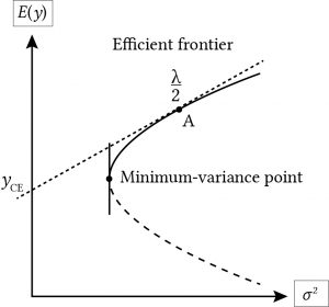
Suppose that we were to draw a line tangent to the relevant section of the EV at point A, representing an investment A. Then the slope of the line at point A would equal the decision maker’s risk coefficient at the point. Furthermore, were we to extend the tangent line to intersect with the vertical axis, the point of intersection would equal the certainty equivalent of the investment.
The Normal Probability Density Function (pdf)
If you have a large enough sample of outcomes from a normal distribution, the distribution will look like a bell-shaped curve.
Figure 15.2. A normal probability distribution that describes probability in areas divided to standard deviations from the mean.
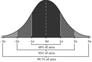
The normal distribution is symmetric about its expected value. The numbers in the graph correspond to standard deviations measured from the mean of the normal distribution. All of the characteristics of the normal distribution are completely described by the mean and variance (or equivalently, the standard deviation). The mean specifies the average value of the rate of return. The probability of getting a return above or below the mean by a certain amount is determined by the size of the standard deviation.
If the returns are normally distributed, there is a 68% chance that the return for any given period will be within one standard deviation of the expected value; a 95% probability that any particular observed return will be within 2 standard deviations of the expected value; and a 99.74% probability that any return will be within 3 standard deviations of the mean. Clearly, the larger the standard deviation, the more spread out the actual returns that occur will be. Suppose the common stock returns we looked at earlier were generated by a normal distribution. We estimated the expected value of the distribution to be r = 18.92% and the standard deviation to be σ(r) = 16.18%. If we were interested in predicting what next year’s return on common stocks will be, we could say that the expected value will be about 18.92%, but, in addition, there is a 68.26% probability that returns will be between 2.74% and 35.1%; a 95.44% probability that returns will be between –13.44% and 51.28%; and a 99.74% chance that the returns will be between –29.62% and 67.46%. The smaller the standard deviation, the less spread out the returns will be and the more accurate the mean will be as a predictor of future returns.
Sampling error. The normal distribution is an important distribution from both a theoretical and a practical standpoint. It is important to note that if you are looking at a small sample of data, its empirically based pdf is likely not to have the shape of a normal distribution even if it is actually generated from a normal distribution. In a small sample, the distribution will have gaps and holes in it and is unlikely have a shape that looks like the true distribution that generated the data. If you keep adding observations from the distribution, eventually the gaps will fill in, and it will start to look like the true distribution that generated the data. The point here is, even if the sample pdf generated by a normal distribution does look like a normal distribution, this may be because the sample size is too small. Therefore, because of its usefulness and tractability, we often assume that our sample pdfs are normally distributed.
Direct and Indirect Outcome Variables
Typically, we connect a risky event ϵ to a random variable y(ϵ). For example, ϵ may represent uncertain prices and y(ϵ) may represent income which depends on uncertain prices ϵ. We will refer to ϵ as the direct outcome variable and y(ϵ) as the indirect outcome variable over which the firm’s utility is defined.
In most risk models, the relationship between ϵ and y(ϵ) is monotonic, if the direct outcome variable goes up (down) so does the indirect outcome variable. If prices increase, so does income; if the variance of ϵ increases, so does the variance of y(ϵ). However, one can easily construct examples in which the linkage is not so direct. For example, suppose the firm faces financial stress and that only very favorable outcomes will permit the firm to meet its cash flow obligations and survive. Under such circumstances, the firm may increase its expected income and its probability of surviving by choosing a strategy that increases its variance of direct outcomes. Consider such a problem by defining an indirect outcome variable w = 0 if the firm fails to survive and w = 1 if the firm survives. In this model the direct outcome variable is y. Then we connect the indirect outcome variable w to the direct outcome variable y by defining a survival income yd and defining w in terms of y as follows:
\[w=\left\{\begin{array}{ll}{0} & {\text { for } \quad y<y_{d}} \\ {1} & {\text { for } \quad y \geq y_{d}}\end{array}\right. \nonumber\]
The ad hoc decision rule can be expressed as:
\[V(y)=\left\{\begin{array}{lll}{U(0)} & {\text { for }} & {y<y_{d}} \\ {U(1)} & {\text { for }} & {y \geq y_{d}}\end{array}\right. \nonumber\]
Since U(0) and U(1) are arbitrarily assigned values, let U(0) = 0 and U(1) = 1. Then, the ad hoc decision rule to be maximized is:
(15.14)
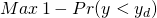
which calls for minimizing Pr(y < yd). This rule is known as Roy’s safety-first rule. When direct outcomes are defined in terms of winning or losing, Roy’s safety-first rule is consistent with an expected utility model.
Of course, one can think of other direct and indirect outcome variable relationships. For example, y could represent uninsured income and w could represent insured income, or y could represent unhedged income and w could represent hedged income, or y could represent income produced without risk reducing inputs and w could represent income produced with risk reducing inputs.
So what have we learned? We learned that risk responses are defined over direct outcome variables. Failure to distinguish between indirect and direct outcome variables may lead us to view responses to indirect outcome variables as risk preferring when they are indeed risk averting.
Firm Responses to Risk
Individuals and businesses all face risky events, including the possibility of losses that leave them less well off than before the outcome associated with the risky event occurred. These outcomes may include you or someone you care about becoming ill or unemployed. Business also face the possibility of losing customers, production failures, declining prices, and loss of financial support.
The next section describes alternative responses to risky events available to firms and individuals. If firms and individuals limit their risk responses described by alternatives on an EV frontier and select risky alternatives consistent with their underlying risk preferences, then they will maximize their certainty equivalent income. Higher risk-averse decision makers will select investments with lower expected values and variances. Less risk-averse decision makers will select investments with higher expected values and variances. If the firm’s current risk position is an expected value-variance combination off the frontier, then the firm’s risk responses may be designed to move the firm closer to a position on the EV frontier.
More to the point, moving up or down its EV frontier involves paying another unit to absorb part or all of its risk (e.g. buying insurance) or changing the relative amount of safe and risky investments in its portfolio.
Someone once claimed that economists can predict the past correctly only 50% of the time. Imagine how successful economists are at predicting future outcomes for risky events? This should suggest that even though we present risk response solutions in closed forms, we should be cautious and explore alternative assumptions and predictions to explore the robustness of our estimates. With that caution in mind, we proceed to explore external risk responses (pay others to absorb our risk) and internal risk responses (change the firm’s holdings of risky and safe investments).
Our discussion of risky and uncertain events and how to measure the probabilities of their outcomes has prepared us to evaluate alternative risk responses including: (1) sharing risk with others through various arrangements including forming partnerships and cooperatives, (2) buying insurance, (3) diversifying one’s holdings of risky investments, (4) purchasing risk reducing inputs, and (5) choosing optimal capital structure. In addition, we will introduce the expected value-variance criterion for ranking alternative risky investments. Finally we will explore how converting risky cash flow to their certainty equivalents can provide the means for introducing risk into PV models so that the homogeneous measures principle applied to risk is satisfied.
Sharing Risky Outcomes
One way to mitigate the impact of adverse outcomes associated with risky events is by forming risk sharing arrangements with others even when they are facing similar risks. The key to successful risk reduction combinations with others is to combine operations that are statistically independent of each other. Statistical independence has a precise meaning, but essentially it means that the expected value of the product of two random variables equals the product of their expected values. In a later section we will discuss combining firms’ operations within other firms whose returns tend to move together.
To make the point that combining units
experiencing independent risky outcomes can mitigate risk, consider
the following. Let x be a random variable with expected
value  and variance
  respectively. Let “a” and “b” equal numerical constants. Then,
define a new random variable:
respectively. Let “a” and “b” equal numerical constants. Then,
define a new random variable:
(15.15)

The variance of y,  ,
is equal to:
,
is equal to:
(15.16)

The explanation for Equation \ref{15.16} is that the variance of the constant “a” or any constant is always zero while the variance of a constant times a random variable is the constant squared times the variance of the random variable.
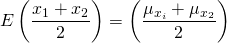
In Equation \ref{15.15} we created a new random variable y by linearly transforming the random variable x. Now consider another way to create a new random variable—by taking the average of two (or more random variables). For example, suppose two businesses were facing independently distributed risky earnings. One business owner faced the random variable x1 and the second business owner faced the random variable x2. Also suppose that the two business owners decided to combine their businesses and agreed that each would receive half of the average earnings. In this process we define a new random variable.
(15.17)

First, recognize that each random variable is multiplied by the constant (1/2). Then each partner would earn on average the expected value
(15.18)
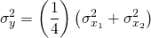
and the variance each owner would face would be the variance of the expected return multiplied by the constant (1/2) squared. The variance of the average earnings each firm would receive, σy2, is equal to:
(15.19)
n the case that the distributions were
identically distributed with expected value and variance of
and ,
each partner would face the same expected value as before,
.
But, the variance of their individual earnings would be  ,
half of what it was before without combining their businesses.
Furthermore, the standard deviation of the earnings each partner
would face would be:
,
half of what it was before without combining their businesses.
Furthermore, the standard deviation of the earnings each partner
would face would be:
(15.20)

And if n partners
joined together, then they would each face the same expected value
as before, but the variance each partner would receive is  .
We now illustrate
these important results.
.
We now illustrate
these important results.
Assume that business one’s earnings are determined by outcomes associated with the toss of a fair coin. If the outcome of the coin toss is tails, the firm pays (loses) $5,000. If the toss is a heads, the firm wins $8,000. Thus, the firm wins either $8,000 or loses $5,000 and earns on average (.5) (–5,000) + (.5) (8,000) = $1500.
The standard deviation of this risky outcomes is:
(15.21)

Furthermore, assuming a normal distribution, 68% of the time, the average outcome will be between the mean and plus or minus one standard deviation: ($1,500 + $6,500) = $8,000 and ($1,500 – $6,500) = –$5,000.
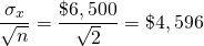
Now suppose that two persons decide to combine their operations and share the average of the outcomes. Then the possible outcomes of two coin tosses are two heads (H, H) which earns on average $16,000 / 2 = $8,000 and occurs with a probability of .25; two tails (T, T) which earns on average –$10,000 / 2 = –$5,000 and occurs with a probability of .25, and one head and one tail (H, T) or one tail and one head (T, H) which both earn on average $3,000 / 2 = $1,500 and each occurs with a probability of .25. The expected value for each of the two players can now can be expressed as:
(15.22)

The two players now receive on average the same as before, $1,500, but consider the standard deviation of the average outcome:
(15.23)

Furthermore, assuming a normal distribution, 68% of the time, the average outcome will be between the mean and plus or minus one standard deviation: ($1,500 + $4,596) = $6,096 and ($1,500 – $4,596) = –$3,096. Note that even though the expected value did not change when outcomes were averaged over two persons, the standard deviation was reduced almost 30%. Also note that the results are in accord with Equation \ref{15.24}:
(15.24)
Now imagine ten persons each facing independent and identical distributed earnings outcomes, then the standard deviation each would face would equal:
(15.25)
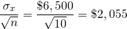
Furthermore, assuming a normal distribution, 68% of the time, the average outcome will range between ($1,500 – $2,055) = –$555.48 and ($1,500 + $2,055) = $3,555. Note that even though the expected value did not change when outcomes were averaged over ten persons, the standard deviation was reduced almost over 70%. Reducing the variability for each person by over 70% by combining ten independent risky events (facing each of 10 independent firms) illustrates the power of reducing risk by sharing independent risky events.
In the previous example we assumed that each
partner contributed an equal share. Now assume two persons decided
to form a partnership and share the risk and expected returns
weighted by their shares contributed to the business. Assume
partner 1 contributed w1 = 30% of the assets
and partner 2 contributed w2 = 70% of the
business. Each partner’s business rate of return can be described
by random variable y1 and
y2 with expected values and variances for
partner one of  and
and  for the first partner and
  and
and  for the second partner. We want to find expected value of the
partnership and each partner’s share of the expected value. Then,
we want to find the variance of the partnership and the variance of
returns each partner would face.
for the second partner. We want to find expected value of the
partnership and each partner’s share of the expected value. Then,
we want to find the variance of the partnership and the variance of
returns each partner would face.
First, to find the expected value of the partnership, we weight each partner’s contribution by the percentage of their contributions. Call the expected return of the partnership E(yp):
(15.26)

Meanwhile, the variance of expected return from the partnership is the sum of the individual variances multiplied by the partners’ shares squared:
(15.27)

Furthermore, the standard deviation of the portfolio is 4.5%. Thus, the partnership earns 11.4% on its investments and faces a standard deviation of returns equal to 4.5% which is less than their standard deviation of returns faced alone equal to 5.0% or 6.0%. Of course, they would have to agree on how to distribute profits, but we assume it would be based on the shares they contributed.
Reducing Risk by Purchasing Insurance
It may be difficult for an individual firm to agree with other independent firms on how to share profits and risk. However, an insurance company that absorbs individual firms’ risk in exchange for an insurance premium can reduce the overall risk by combing the risk facing large numbers of individual firms. Furthermore, by carefully selecting businesses from different geographic areas and of different types, the risk absorbed by individual firms can be close to negligible.
For most individuals and businesses, insurance offers a way to reduce their risk when other measures are not available. Insurance is a practical arrangement by which a company or government agency provides compensation for a wide variety of losses and adverse outcomes. For example, we can purchase health insurance in case we become ill, fire insurance in case of a fire, term and whole life insurance for our heirs if we die, revenue insurance in case our expenses exceed income, trip insurance in case our flight gets canceled, and almost any other adverse outcome as long as we are willing to pay someone to assume the possibility of loss. This kind of insurance, discrete disaster event insurance, is described next.
Discrete disaster event insurance.
Consider a firm with wealth comprised of a risky asset, whose value
is W in the best state of nature and zero in the worst
state of nature, and risk-free assets valued at
W0 regardless of the state of nature. An
insurance company is willing to absorb the risk of possible losses
of wealth in exchange for an insurance premium  .
The firm must determine the maximum insurance premium
.
The firm must determine the maximum insurance premium  it can pay to avoid a disaster without reducing the level of its
certainty equivalent wealth below the level attained with no
insurance coverage. The firm can increase its certainty equivalent
income by purchasing insurance if
it can pay to avoid a disaster without reducing the level of its
certainty equivalent wealth below the level attained with no
insurance coverage. The firm can increase its certainty equivalent
income by purchasing insurance if  .
.
Suppose the firm is considering a comprehensive
fire insurance policy and W represents the value of the
firm’s flammable property being insured. To the find the maximum
insurance premium
that the firm can pay without reducing its certainty equivalent
income, we form the decision matrix displayed in Table 15.2.
The matrix has two possible states of nature, two
choices, and four different possible outcomes. The states of nature
are (1) a fire state s1, and (2) a no-fire
state s2 . The choices are buy insurance
(choice A1) and remain uninsured (choice
A2). If choice A1 is
selected, the outcome in both states s1 and
s2 is initial wealthy W +
W0 less an insurance premium .
This result is obtained because if a fire does occur, the insurance
company reimburses the firm for its losses and receives a risk
premium. If there is no fire, the insurance company pays for no
losses while still earning the insurance premium. In both states
the firm purchasing insurance pays a premium. If, on the other
hand, the firm decides to remain uninsured (choice
A2) and no fire occurs, the firm will be left
with both its safe wealth W0 and its risky
wealth W and will have saved the insurance premium because
it didn’t purchase insurance. However, if a fire does occur, the
firm will lose its risky wealth W. These results are
summarized below.
Table 15.2. Decision Matrix for Insurance Versus No Insurance with a Discrete Disaster Outcome.
| Choices | |||
| States of nature | Probability of outcomes | A1 (buy insurance) outcomes | A2 (Don’t buy insurance) outcomes |
| (s1) fire | 0 < p < 1 |
 |
 |
| (s2) no fire | 1 – p |
|
 |
If the probability of fire is p and the probability of no fire is 1 – p, the expected values of the two choices E(A1) and E(A2) are:
(15.28)
And
(15.29)

The difference between E(A1) and E(A2) can be expressed as:
(15.30)

If the decision maker was risk neutral and
decided between options based on their expected value, the maximum
the client would pay for the fire insurance would be  ,
and as long as
,
and as long as  the client would be better off purchasing insurance than not
purchasing insurance.
the client would be better off purchasing insurance than not
purchasing insurance.
To illustrate, suppose that the flammable
property was W = $100,000 and p = 1%. Then, the
most a client could pay and break-even based on his or her expected
values would be pW = (.01)($100,000) = $1,000. If an
insurance policy was available for less than $1,000, the client
would be advised to purchase the insurance. Suppose the client is
risk averse and lays awake at night worrying about the possibility
of a fire, and perhaps the client is willing to pay an additional
insurance premium based on some function of p and
W equal to U(p,W) $150 to know
that, no matter what, the outcome will be  .
.
Revenue insurance. One for the most important forms of insurance available to individual and firms is revenue insurance. The general principles of revenue insurance can be complicated. We describe a simplified version of revenue insurance with discrete outcomes.
Suppose an outcome from a crop operation is a
risky event with three possible outcomes: normal income y,
reduced income  where
where  is a percentage between one and zero, or a failed crop resulting in
y = 0. Let the probability of y be
p1. Let the probability of
be p2. And let the probabilities of a failed
crop and zero income be (1 – p1 –
p2).
is a percentage between one and zero, or a failed crop resulting in
y = 0. Let the probability of y be
p1. Let the probability of
be p2. And let the probabilities of a failed
crop and zero income be (1 – p1 –
p2).
The insurance provided does not fully compensate farmers for their losses for moral hazard reasons; they want the farmers to experience some losses for not producing a normal crop.
As a result, lost revenues are only compensated
by  percent. Furthermore, there is a complicated process to determine
what is a normal yield that produces y. If a failed crop outcome
occurs, the firm receives
percent. Furthermore, there is a complicated process to determine
what is a normal yield that produces y. If a failed crop outcome
occurs, the firm receives  or
percent of what it normally earns. If a partial crop outcome
occurs, then the firm also earns
because the insurance company pays
of the firm’s lost earnings equal to
or
percent of what it normally earns. If a partial crop outcome
occurs, then the firm also earns
because the insurance company pays
of the firm’s lost earnings equal to 
To describe the revenue insurance program described above we construct Table 15.3.
Table 15.3. Decision Matrix for Revenue with Insurance Versus no Insurance with Discrete Outcomes.
| Choices | |||
| States of nature | Probability of outcomes | A1 (buy insurance) outcomes | A2 (Don’t buy insurance) outcomes |
| (s1) full crop | p1 |
 |
 |
| (s2) partial crop | p2 |
 |
|
| (s3) crop failure | (1 – p1 – p2) |
 |
0 |
To solve for
we equate the expected value for the two choice options:
(15.31)

And solving for the insurance premium
we find:
(15.32)
To illustrate, suppose  and
and  so that
  Assume that the probability of a normal income is 60%, the
probability of a partial crop and a reduced income is 30%, and the
probability of a complete crop failure and no income is 10%.
Finally, assume that your revenue insurance policy covers
= 80% of lost revenue. We restate these conditions in Table 15.4
and then solve for the break-even insurance premium
Assume that the probability of a normal income is 60%, the
probability of a partial crop and a reduced income is 30%, and the
probability of a complete crop failure and no income is 10%.
Finally, assume that your revenue insurance policy covers
= 80% of lost revenue. We restate these conditions in Table 15.4
and then solve for the break-even insurance premium 
Table 15.4. Decision Matrix for Revenue Insurance Versus No Insurance with Discrete Outcomes.
| Choices | |||
| States of nature | Probability of outcomes | A1 (buy insurance ) outcomes | A2 (Don’t buy insurance) outcomes |
| (s1) full crop | p1 = 60% |  |
|
| (s2) partial crop | p2 = 30% | 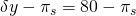 |
|
| (s3) crop failure | (1 – p1 – p2) = 10% | 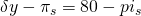 |
0 |
Finally, we solve for the break-even insurance
premium 
(15.33)

In other words, a manager could afford to pay up to 17% of its normal income as revenue insurance under the conditions described in Table 15.3.
Diversification of Firm Investments
Investors rarely hold investments in isolation. Indeed, holding a single investment by itself may be very risky. Most investors attempt to reduce risk by holding a portfolio of (two or more) investments. Adding a risky investment to a portfolio of investments may actually decrease the risk of the portfolio without adversely affecting the expected return on the portfolio. We illustrate the point that adding risky investments to one’s portfolio may decrease risk with an example.
Umbrellas and sunglasses. Suppose that on any given day there are three possible weather outcomes: there may be rain, there may be a mix of clouds and sun, and there may be bright sunny skies. For simplicity, assume that the probability of each outcome is 1/3. A firm whose outcomes depend on the weather state can invest in umbrellas or sunglasses or a mix of the two. Both investments in umbrellas and sunglasses earn an expected rate of return equal to 10%. These results are summarized in Table 15.5 below:
Table 15.5. Expected Returns and Variances on Investments in Sunglasses and Umbrella
| Weather states i = 1,2,3: | Probability of weather states | Random Returns on Sunglasses in the ith weather state: riS | Random Returns on Umbrellas in the ith weather state: riW | Return on portfolio |
| Rain | 1/3 | 0% | 20% | .5(0) +.5(20%) = 10% |
| Mix clouds and sunshine | 1/3 | 10% | 10% | .5(10) +.5(10%) = 10% |
| Sunny | 1/3 | 20% | 0% | .5(20) +.5(0%) = 10% |
| Expected return on investments: | E(riS) = (1/3)(0% + 10% + 20%) = 10% | E(riW) = (1/3)(20% + 10% + 0%) = 10% | .5E(riS) + .5E(riS) = (1/3)(10% + 10% + 10%) = 10% | |
| Standard deviation of returns: | 8.16% | 8.16% | 0% | |
Notice that when it rains, return on umbrellas is favorable (20%) but the return on sunglasses is low, 0%. The reverse is true when there are bright sunny skies; the return on umbrellas is low (0%) while the return on sunglasses is favorable, 20%. The standard deviation for both investments equals:
(15.34a)

Now assume that the firm diversified and created a portfolio in which 50% of its investments were in sunglasses and the other 50% were in umbrellas. The results are described in the last column of Table 15.5. Notice that the return in each state is 10% because when returns on low on sunglasses, return on umbrellas are favorable and vice versa. Note also that while each individual investment has a standard deviation of returns equal to 8.16%, the return on the portfolio is constant and the standard deviation of portfolio returns is zero.
(15.34b)

This is an extreme example of how adding a risky investment may actually decrease the firm’s risk. However, this favorable result occurred because the returns on umbrellas and sunglasses were perfectly and negatively correlated.
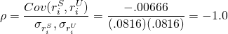
Covariance measures. To be perfectly and negatively correlated means that returns on one investment is above its mean by exactly same amount as the other investment is below its mean in the same state. One measure of correlation between two random variables is the covariance measure. Using the notation from the umbrellas and sunglasses example, we define the covariance as:
(15.35)
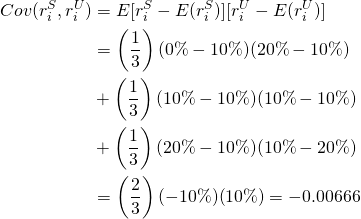
Notice that the covariance is similar to a variance measure except that instead of a deviation from the expected value being squared, the deviation for both variables in the same state are multiplied, so the covariance measures whether the two variables are moving in opposite directions from their means (negative covariance) or whether the two variables are moving in the same direction from their means (positive covariance). To emphasize the difference between variance and covariance measures, when calculating variance, we squared deviations from the mean, and as a result all variances are positive. In contrast, deviation in covariance measures are not squared which allows them to be positive or negative. Note that the first and third term in the covariance calculation in Equation \ref{15.35} were negative while the second term was zero. Thus, the covariance of investments in sunglasses and umbrellas is negative.
Obviously the sunglasses and umbrellas example is
simplified to illustrate a point, that risk is completely
eliminated because the returns from the two investments have
perfect negative correlation. The level of correlation between
returns is measured by the correlation coefficient  defined as:
(15.36)
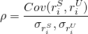
Thus, in our example, the correlation coefficient is negative one:
(15.37)
Obviously, other things being equal, we would prefer to add investments to our portfolio that are negatively correlated with our overall portfolio returns.
Let’s return to our investigation of the partnership, only this time allow for a single firm to consider its rate of return on its portfolio of investments. Assume that it has two investments and the percent of the total portfolio invested in each investment is indicated by a weight w1 and w2 that sum to one. The expected value for the firm’s portfolio can be expressed as before:
(15.38)
Now consider the variance of the investor’s portfolio. If the investments are represented by independent random variables, the portfolio variance is as before—the weighted sum of the individual variances. When the investments are not independent, the portfolio variance also includes a covariance term. We can write the variance of the portfolio allowing for dependence between the two investments as:
(15.39)

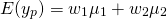
We now apply our portfolio approach to the umbrellas and sunglasses example. Recall that both investments earned an expected rate of return of 10% and their standard deviations were both equal to 8.16%. If the firm divided their portfolio between the two investments, then we would write the expected value and variance of the portfolio as:
(15.40)

And we write the portfolio variance as:
(15.41)
In this special example, that the returns on sunglasses and umbrellas moved in perfectly opposite direction means that combining investments in both eliminated the variability of returns on the firm’s portfolio.
Beta coefficients and risk diversification. An important risk concept applied to securities markets but which also has application to the firm is the beta coefficient (β). The beta coefficient is a measure associated with an individual investment which reflects the tendency of an investment’s returns to move with the average return in the market. Applied to the individual firm, the beta coefficient measures the tendency of an individual investment’s returns to move with the average return on the firm’s portfolio of investments.
To explain beta coefficient, suppose we have past rate of return observations rtj on a potential new investment and on the firm’s portfolio of returns rtp in time period t. Table 15.6 summarizes our observations:
Table 15.6. Observations of Returns on the Firm’s Portfolio of Investments rtp and on a Potential New Investment (a Challenger).
| Time t | Observed returns on the firm’s portfolio over time rtp | Observed returns on a potential new investment for the firm’s rtj |
| 2012 | 10% | 7% |
| 2013 | 6% | 8% |
| 2014 | 7% | 5% |
| 2015 | 3% | 2% |
| 2016 | 5% | 3% |
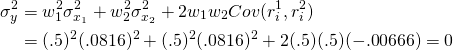
Another way to represent the two rates of return measures and their relationship to each other is to represent them in a two dimensional scatter graph.
We may visually observe how the two sets of rates of return move together by drawing a line through the points on the graph in such a way as to minimize the squared distance from the point to the line. Our scatter graph is identified as Figure 15.3.
Figure 15.3. Scatter Graph of Returns on the Firm’s Portfolio of Investments and Returns on the Potential New Investment
The relationship between the returns on the new investment and the firm’s portfolio can be expressed as:
(15.42)
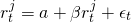
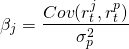
Notice that the equation above describes the straight line drawn through the point plus the vertical distance from the line to each point. The slope of the line is the beta coefficient β and tells us how the returns on the portfolio and potential new investment have moved together in the past. We can find the equation for this line using a statistical method called “least squares” regression analysis. The method essentially finds a line so that the average squared deviations from the line, εt2, are minimized. The formula for beta is equal to the covariance between the returns on the new investment rtj and the returns on the firm’s portfolio rtp over some time period divided by the variance of portfolio returns:
(15.43)
Fortunately, the calculations for the beta coefficient as well as the coefficients in Equation \ref{15.16} can be found using Excel.[2] We find the beta coefficient and the coefficients for Equation \ref{15.16} using the data in Table 15.6.
The estimated equation for the line is:
(15.44)

Diversifiable and non-diversifiable risk. Assume a beta coefficient of minus one (–1). This would mean that for a 10% increase (decrease) in the firm’s overall rate of return, that the expected rate of return on the potentially new investment decreases (increases) by 10%. Like investments in sunglasses and umbrellas, a sufficient investment in the new investment would eliminate the firm’s risk. Thus, a beta of –1 means that all of its risk can be diversified. In contrast, assume a beta coefficient of one. This would mean that for a 10% increase (decrease) in the firm’s overall rate of return, that the expected rate of return on the potentially new investment increases (decreases) by 10%. Unlike investing in sunglasses and umbrellas, adding the potentially new investment to the firm’s portfolio of investment only accentuates its risk, and the new investment has no potential to diversify the firm’s overall risk.
Purchase Risk Reducing Investments
It is useful to distinguish between two primary reasons for investing: first, to increase expected earnings for the firm and second, to reduce the variability of earnings. If one can increase expected returns without increasing variance of return, certainty equivalent income has increased. If one can reduce variance of returns without also reducing expected returns, certainty equivalent income has increased. See Equation \ref{15.12}. Of course if from one’s current expected value-variance position, one could increase one’s expected value of returns without increasing the variance of returns—or if one could reduce one’s variance without also reducing one’s expected value—then the firm would be in an inefficient expected value-variance position off the EV frontier. However, we can identify investments whose primary purpose is to reduce variability even though they alter expected incomes. We call these risk reducing investments. We analyze risk reducing inputs using the certainty equivalent income model described in Equation \ref{15.12} that accounts for both variance and expected value in the ranking criterion.
We will illustrate risk reducing investments with
a case study involving an irrigation investment. Consider a firm
facing five moisture states with an equally likely chance of
occurring: normal, low stress, moderate stress, high stress, and
drought. The returns per acre with and without the irrigation
system are reported in Table 15.7. The annualized cost of the
irrigation system, which is expected to have a 20 year life and no
liquidation value, is  per acre. We assume the defender’s IRR associated with the
certainty equivalent cash flow stream to be 8%.
per acre. We assume the defender’s IRR associated with the
certainty equivalent cash flow stream to be 8%.
Table 15.7. Returns per Acre under Alternative Moisture States with and without an Irrigation System.
| Moisture states | Probability of moisture states | Return per acre without the irrigation investment riw/0 | Return per acre with the irrigation system riw minus irrigation costs per acre π |
| Normal | 20% | $128.00 | $113– π |
| Low stress | 20% | $105.00 | $100 – π |
| Moderate stress | 20% | $90.00 | $80 – π |
| High stress | 20% | $75.00 | $75 – π |
| Drought | 20% | $50.00 | $70– π |
| Expected returns | $89.60 | $87.60 | |
| Standard deviation of returns | $26.43 | $16.28 | |
Assume that
is $15 per acre. Then the expected value of the crop production per
acre without irrigation is still $89.60 and greater than $87.60. If
the decision maker were risk neutral, he or she would not invest in
the irrigation system. Allow that the decision maker is risk averse
and chooses between investments based on their certainty equivalent
incomes rather than the difference in their expected values. If
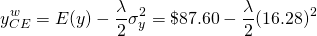
this were the case, then the certainty equivalent income without
irrigation is:
(15.45)

In contrast, the certainty equivalent income with the irrigation system is:
(15.46)
We cannot decide between the two systems because
one has a higher expected value and the other has a lower variance.
It all depends on how risk averse the decision maker is. Recall
that  reflects the decision maker’s preferred trade-off between expected
return for variance. The break-even λ in this case is found by
equating the two certainty equivalent incomes:
reflects the decision maker’s preferred trade-off between expected
return for variance. The break-even λ in this case is found by
equating the two certainty equivalent incomes:
(15.47)
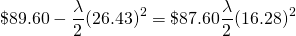
and solving for :
(15.48)
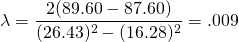
Thus, all decision makers more risk averse than
is reflected by the risk aversion coefficient of
= .009 will be earning a lower expected value on average than would
be earned without the irrigation system.
Choosing an Optimal Capital Structure
Leverage and risk. In an earlier chapter, we used leverage as a measure of the firm’s risk without explicitly stating the connection. We now make the connection explicit by reconsidering equation 8.5 and making one adjustment. The adjustment is that since we only consider realized capital gains when finding ROA–IRR, we ignore unrealized capital gains (V1 – V0) which allows us to rewrite equation 8.5 as:
(15.49)
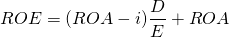
In Equation \ref{15.49}, note the leverage ratio D/E and that it multiplies the difference between the ROA and the average interest rate i. And now we return to a risk principle introduced earlier—that multiplying a random variable by a constant, in this case the leverage ratio, increases the variance of the random variable by the constant squared. Consider the application of this principle.
Suppose the random variable ROA is described by pdf f(rROA) with expected value rROA and variance σ2. Now suppose that we were to multiply the random variable ROA by some scalar, say 2. Then the expected value of the random variable would be 2rROA and the variance would be 22σ2, or 4σ2.
In Equation \ref{15.49}, the debt-to-equity ratio is the scaler that multiplies and exaggerates the difference between rROA and i. To illustrate, suppose that ROA can take on values of –8%, –3%, 3%, 5%, and 12% and i = 3%. Then in Table 15.8 we find ROE for leverage ratios of 0, 2, 5, and 10.
Table 15.8. ROEs whose Expected Values and Standard Deviations depend on Leverage Ratios.
| Values of the random variable ROA (i = 3%) | ROE values for alternative Leverage Ratios (L = D/E) and values of the random variable ROA | |||
| L = 0 | L = 2 | L = 5 | L = 10 | |
| –8% | –8% | –30% | –63% | –118% |
| –3% | –3% | –15% | –33% | –63% |
| 3% | 3% | 3% | 3% | 3% |
| 5% | 5% | 9% | 15% | 25% |
| 12% | 12% | 30% | 57% | 102% |
| Standard deviations for ROEs associated with each leverage ratio L | ||||
| Expected values | 1.8 % | –.6% | –4.2% | –10.2% |
| Standard deviation σ | .077 | .23 | .460 | .843 |
The first thing to note about the outcomes in Table 15.8 is that whenever the ROA exceeds the average interest rate i, that ROE > ROA. For example, for a leverage ratio of 2 and an ROA of 5%, ROE is 9%. The second point to observe is that even though the E(ROA) > 0, as the leverage ratio increased, the E(ROE) was mostly less than zero. In other words, the effect of leverage was more pronounced when the ROA < i than when ROA > i. Another thing to note is that if the ROA outcome is –8% and the firm has a leverage ratio of 10, it loses 118% of its equity. In other words, one unfavorable outcome with a high leverage ratio can destroy the firm. Finally, due to the cost of debt that must be paid regardless of ROA outcomes, ROA’s less-than-average cost of debt with high leverage ratios have significant adverse effects on the firm’s equity. Thus, we conclude that a high leverage ratio, even though it can exaggerate unusually high ROA outcomes, is still a risky state for the firm. For that reason, many firms view leverage reduction as an important strategy for reducing the riskiness of the outcomes they face.
Capital structure. A firm’s capital structure is its combination of debt and equity used to finance its overall operations and growth. The small to medium-size firm may finance its overall operations and growth by using long-term debt, equity, and notes payable. We will discuss the small to medium-size firm’s optimal capital structure using a simplified expected value-variance (EV) profit model.
In our simplified model, we let the firm’s assets
A be funded by a combination of debt D and equity
E. We let  be the stochastic rate of return on the firm’s assets whose
variance is
be the stochastic rate of return on the firm’s assets whose
variance is  and whose expected rate of return is ra. We let
the average non-stochastic cost of debt per dollar be represented
by the variable iD. The firm decision maker’s
risk-return trade-off is measured by
and whose expected rate of return is ra. We let
the average non-stochastic cost of debt per dollar be represented
by the variable iD. The firm decision maker’s
risk-return trade-off is measured by 
We represent the firm’s stochastic profits
 to equal the stochastic rate of return on assets times assets less
the firm’s average cost of debt times the firm’s debt. Then we
substitute for assets A the sum of debt D plus
equity E and collect like terms and express the stochastic
results in Equation \ref{15.50}.
to equal the stochastic rate of return on assets times assets less
the firm’s average cost of debt times the firm’s debt. Then we
substitute for assets A the sum of debt D plus
equity E and collect like terms and express the stochastic
results in Equation \ref{15.50}.
(15.50)

We write the expected value of stochastic profits as:
(15.51)

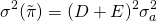
We write the variance of profits as:
(15.52)
Finally, we substitute the expected value and
variance of profits into Equation \ref{15.51} to find the firm’s
certainty equivalent of profits  that we refer to as the EV model.
(15.53)

Finding the firm’s optimal capital
structure.[3]
Having our EV model defined over the expected value and variance of
profits and accounting for the decision maker’s risk attitudes, we
use calculus to find the optimal debt level by differentiating the
certainty equivalent function
with respect to D.
(15.54)
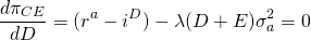
The second order conditions are satisfied allowing us to solve for the optimal debt D* (assuming fixed equity). We find the optimal debt D* to equal:
(15.55)
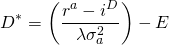
Equation (15.55) reveals an interesting detail. If the cost of debt equals the expected return on assets, the firm holds negative debt—preferring to lend out its equity at a safe rate iD rather than earning a stochastic return on firm assets.
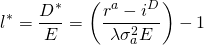
Dividing Equation \ref{15.55} by the firm’s equity E, we can find its optimal leverage ratio l* equal to:
(15.56)
We illustrate Equation \ref{15.56} using HQN’s
data. We substitute for ra the ROA value equal
to 6.5% (equation 5.13), the average cost of debt
iD equal to 6% (equation 5.21), equity
E equal to $8,000 (Table 4.1), the risk aversion
coefficient calculated in Equation \ref{15.48} equal to .009, and
finally, we let the standard deviation—the amount that returns on
assets vary on average—equal 1.25% or .0125 that we square to find
the variance of profits  equal to .000156. Making the substitutions for the variables in
Equation \ref{15.56} we find the firm’s optimal leverage ratio
equal to:
equal to .000156. Making the substitutions for the variables in
Equation \ref{15.56} we find the firm’s optimal leverage ratio
equal to:
(15.57)

compared to the firm’s actual leverage ratio of 4.0.
Changing variables affecting the optimal capital structure. We can imagine how the optimal leverage would change in response to changes in the value of the variables included in Equation \ref{15.57}. In other words, we ask: how would the optimal leverage change if the value of one of the variables in Equation \ref{15.57} changed? We can infer the answer to this question by looking at changes in the optimal leverage ratio in response to a change in one of the variables holding the other variables constant.
Increasing the expected value of asset returns
ra makes it more profitable to use borrowed
funds and increases the optimal leverage ratio. Increasing the
average cost of debt iD makes using debt less
profitable and reduces the optimal leverage ratio. As a decision
maker becomes more risk averse, represented by an increase in the
risk aversion coefficient ,
the decision maker is less willing to risk losing equity with an
unfavorable outcome and reduces leverage. As the firm’s equity
increases, it can achieve the same risk return combination with
less debt and the optimal leverage ratio decreases. Finally, as the
variance of return on firm assets
increases, the firm reduces its leverage ratio to return to its
preferred trade-off between equity and debt.
In addition to describing how the firm’s finds its optimal capital structure in response to changes in the value of the variables that determine the optimal capital structure, we create Table 15.9. Columns in Table 15.9 include the list of variables, their original values for HQN, a column showing increased values of the variables, the revised optimal leverage ratio, and the change in the optimal leverage ratio compared to the original optimal leverage ratio of 3.45.
Table 15.9 Optimal leverage ratios and changes in the optimal leverage ratio in response to increases in one of the variables in Equation \ref{15.57} holding the other variables constant.
| Variable | Original value | Increased value | Revised optimal leverage ratio | Change in the optimal leverage ratio |
| ra | 6.5% | 7.0% | 7.903134 | 4.45 |
| iD | 6% | 6.5% | (1) | (4.45) |
|
.009 | .001 | 3.01 | (.44) |
|
0.000156 | .000175 | 2.97 | (.48) |
| E | $8,000 | $9,000 | 2.96 | (.49) |
Summary and Conclusions
Some sage is reported to have said that only death and taxes are certain. If that statement is anywhere close to being true, then risk and uncertainty fill the world we live in and try to manage. One important step toward managing the outcomes of risky events is to understand the tools that have been developed to report and measure it. In this effort, precision is not expected. It is best to explore the influence of risk in a variety of settings and assumptions.
The second thing to note about risk, emphasized in the irrigation example, is that individual risk preferences may have significant effects. As a result, two individuals facing the same investment opportunities may make different choices because of the different risk preferences. As a result, it is important for managers to explore their own risk preferences and apply them when making risky decisions.
Questions
- This question has several parts.
- What is the difference between a sample of observations and the population of possible values?
- Explain the difference between an expected value and variance (standard deviation) calculated from a sample and the expected value and variance (standard deviation) of a population.
- Find the expected value and variance (standard deviation) for the numbers 5, 8, –3, 9, and 0. Assume each number has an equally likely chance of being observed.
- Find the expected value and population variance (standard deviation) for the numbers 5, 8, –3, 9, and 0 if their probability of occurring were .1, .2, .4, .2, and .1 respectively.
- Compare the results obtained in parts c and d.
- Return to Table 15.1 in the text. Suppose that the investor decided to invest half of her assets in investment A and half in investment B. Describe the random variable for the combined investment. Then describe its pdf, expected value, and variance (standard deviation). Based on the respective expected values and variances for investment A, investment B, and the combined investment—which would you prefer, assuming you are risk averse?
- Assume two people decide to form a partnership and share the risk and expected returns based on their shares contributed to the business. Assume partner 1 contributed 40% of the assets and partner 2 contributed 60% of the assets. Each partner’s business can be described by random variables y1 and y2 with expected values and variances of μ1 = 8% and σ12 = 0.006 for the first partner and μ2 = 12% and σ22 = .007 for the second partner. Find the expected value standard deviation of the partnership.
- Assume that Kelly wants to provide for her heirs in case she dies during the coming year. Therefore, she purchases a term life insurance policy that pays $1,000,000 in case she dies in return for an insurance premium of $800. Assuming Kelly is risk neutral, what must Kelly assume is the probability of her death in order for her to purchase the insurance policy?
- Assume the conditions described in Table 15.3 except allow for the insurance coverage δ to increase from 80% to 85%. Find the increase in the break-even insurance premium.
- Assume the conditions described in Table 15.4. Also assume that instead of purchasing revenue insurance the investor could purchase an irrigation system that would increase the probability of a normal revenue income year from 60% to 75%, reduce the probability of a reduced income year from 30% to 20%, and reduce the probability of zero income from 10% to 5%. What would be the most that the manager could pay to reduce its risk through the purchase of an irrigation system and still be as well as he was before? (Hint: compare the value provided by the irrigation system less the cost of the irrigation system compared to the outcomes without an irrigation system.)
- One of the differences between the purchase of an irrigation system and revenue insurance is that one has to purchase revenue insurance each year while the irrigation system continues to provide risk reduction services during its useful life. If the irrigation system described in the previous question were available for 10 years and the discount rate were 8%, what is the NPV of the irrigation system?
- Use the data in Table 15.5 to find the beta coefficient for the investment in umbrellas and sunglasses.
- A firm has two investments in its portfolio. The historical rates of return on the two investments are reported below. Find the expected rate of return for the firm’s portfolio, the covariance between the two investments, and the variance of the portfolio returns. Rank investment 1, investment 2, and the combined investment using the EV criterion.
Table Q15.1. Observations of Returns on the Firm’s Two Investments
| Time t | Observed returns on investment one. | Observed returns on investment two. |
| 2012 | 10% | 7% |
| 2013 | 6% | 8% |
| 2014 | 7% | 5% |
| 2015 | 3% | 6% |
| 2016 | 5% | 4% |
- The authors thank Jack Meyer for the thumbtack example of an uncertain event. ↵
- The linear regression equation that includes the Beta coefficient is found in Excel by first plotting a scatter diagram and then hovering over a data point in the graph. A complete discussion of linear regression models is outside the scope of this class. ↵
- This section uses calculus to find the firm’s optimal debt level and its optimal capital structure or leverage ratio (D/E). Those not interested in the derivation may skip to the next section without loss of continuity in the discussion. ↵