
12: Homogeneous Rates of Return
- Page ID
- 12757

After completing this chapter, you should be able to: (1) construct present value (PV) models using multi-period equivalents of an accrual income statement (AIS); (2) find multi-period before and after-tax rates of return by solving internal rate of return (IRR) models; and (3) solve practical investment problems using present value model templates that are consistent with generalized AIS construction principles.
To achieve your learning goals, you should complete the following objectives:
- Describe the similarities and differences between an AIS and IRR PV models.
- Construct multi-period IRR models by generalizing AIS earning measures.
- Demonstrate that before and after-tax return on assets (ROA) and return on equity (ROE) measures derived from an AIS are equivalent (equal) to rate of return measures derived from multi-period (one-period) IRR models.
- Learn how to divide the PV model construction process into three phases: the acquisition phase, the operating phase, and the liquidation phase.
- Construct net present value (NPV) models by discounting a challenger’s cash flow using a defender’s IRR.
- Show how NPV models that discount a challenger’s cash flow and changes in operating and capital accounts with a defender’s IRR can be used to rank defenders and challengers.
- Develop PV construction skills by using Excel templates.
Introduction
In this chapter, we find before and after-tax one-period rates of return on assets and equity by calculating cash flow and changes in operating and capital accounts. Operating accounts include accounts receivable (AR), inventories (Inv), accounts payable (AP), and accrued liabilities (AL). Depreciation (Dep) plus changes in realized capital gains measure changes in the firm’s capital account.
Next, we point out the similarities and differences between AIS and IRR PV models. Then using HQN data introduced in Chapter 4, we derive ROA and ROE measures in an AIS and a one-period IRR model demonstrating that the two models produce equal results. Next, we show how AIS construction principles guide the construction of multi-period IRR PV models.
We acknowledge that AIS and IRR models are descriptive tools. They describe the rate of return on assets or equity of the firm (industry or sector) or investment. Prescriptive PV models that produce investment recommendations require that we combine before and after-tax ROA and ROE measures for a defending investment, the investment owned by the firm, and cash flow and changes in operating and capital accounts for a challenging investment, a potential replacement for the defending investment. Continuing, we divide the IRR and NPV PV model construction into three stages: the acquisition phase, the operating phase, and the liquidation phase. Finally, we operationalize the construction of PV models by introducing a generalized PV model.
Accrual Income Statement (AIS) versus Internal Rate of Return (IRR) Present Value Models
Consider the similarities and differences between an AIS and IRR models.
Descriptive versus prescriptive focus. An AIS generates one-period before and after-tax ROA and ROE. IRR models generate one or multi-period before and after-tax IRRA and IRRE that estimate average rate of return measures on assets and equity respectively. One-period IRRA and IRRE are equal to ROA and ROE AIS measures respectively. However, using multi-period IRR models we can find IRRA and IRRE that estimate average before and after-tax rates of return over several periods for which there are no AIS equivalent measures. However, one-period AIS construction processes can guide the construction of multi-period IRR models.
IRR models like AIS are descriptive in nature—they do not enable us to rank firms or investments unless we compare them to other firms or investments’ rates of return. In contrast, NPV PV models can rank investments because they contain information about two investments, a defending and a challenging investment. A defending investment is one in use. A challenging investment is a potential replacement for a defending investment. NPV models represent a defending investment by its IRR. NPV models represent a challenging investment by its cash flow and changes in its operating and capital accounts over one or more periods. Maximum bid (minimum sell) PV models are variations of NPV models that find break-even investment prices that make the firm indifferent between a defender and a challenger. A positive (negative) NPV infers that the challenger earns a higher (lower) rate of return than does the defender that it replaces.
Past versus future time focus. Most of the time, an AIS measure cash flow and changes in operating and capital accounts resulting from financial and production activities already completed or in the process of being completed. Of course, it is possible to forecast future coordinated financial statements (CFS) by predicting future values of exogenous variables or by changing control variables in the CFS. Multi-period IRR models, on the other hand, are forward looking, attempting to measure anticipated cash flow and changes in operating and capital accounts resulting from projected future financial and production activities.
The firm versus an investment. An AIS focuses on finding returns on the firm’s assets and equity. Meanwhile, IRR models focus on finding the rate of return on an investment. We may say that the focus of an AIS is the firm while the focus of PV models is an investment.
Measuring returns to assets and equity. We can divide returns to assets and equity into three categories:
- cash flow during the period(s) of analysis,
- changes in the firm’s noncash operating accounts; and
- changes in the firm’s capital accounts.
Liquidation of noncash operating and capital accounts. Both AIS and IRR models include the liquidated value of noncash operating and capital accounts. An AIS includes the liquidated value of accounts at the end of one-period. IRR models include the liquidated value of operating and capital accounts at the end of the analysis that may be one or several periods. Liquidated values depend on what the next owners of the operating and capital accounts are willing to pay to acquire them.
So what have we learned? We learned that before and after-tax ROE and ROA derived from AIS and one-period IRR models are equal. In addition, we learned that AIS construction principles can guide the construction of multi-period IRR models. Finally, we learned that rate of return measures derived from AIS and IRR models are descriptive and that we can build prescriptive PV models by combining IRR measures from a defending investment and cash flow and changes in operating and capital accounts for a challenging investment.
Finding Changes in Assets and Equity
We now describe how to find cash flow and changes in operating and capital accounts using AIS and IRR models. Consider the AIS for HQN in Table 4.6 in Chapter 4 and repeated here as Table 12.1. Notice that we organize AIS into total revenue and total expenses. Then, after adjusting for interest, taxes, and dividend/owner draw, we find Addition to Retained Earnings.
Table 12.1. 2018 Accrual
Income Statement for HQN.
Open HQN Coordinated Financial Statement in MS Excel
| ACCRUAL INCOME STATEMENT | ||
| DATE | 2018 | |
| + | Cash Receipts | $38,990 |
| + | Change in Accounts Receivable | ($400) |
| + | Change in Inventories | $1,450 |
| + | Realized Cap. Gains/Depr. Recapture | $0 |
| Total Revenue | $40,000 | |
| + | Cash Cost of Goods Sold | $27,000 |
| + | Change in Accounts. Payable | $1,000 |
| + | Cash Overhead Expenses | $11,078 |
| + | Change in Accrued Liabilities | ($78) |
| + | Depreciation | $350 |
| Total Expenses | $39,350 | |
| Earnings Before Interest and Taxes (EBIT) | $650 | |
| – | Less Interests Costs | $480 |
| Earnings Before Taxes (EBT) | $170 | |
| – | Less Taxes | $68 |
| Net Income After Taxes (NIAT) | $102 | |
| – | Less Dividends and Owner Draw | $287 |
| Addition to Retained Earnings | ($185) | |
Equation (12.1) summarizes the AIS statement in Table 12.1. It equates total revenue to cash receipts (CR) plus changes in accounts receivable (∆AR) plus change in inventory (∆Inv) plus realized capital gains/depreciation recapture (RCG). It equates total expenses to cash cost of goods sold (COGS) plus changes in accounts payable (∆AP) plus cash overhead expenses (OE) plus changes in accrued liabilities (∆AL) plus the change in the book value of capital assets or depreciation (Dep).
The difference between total revenue and total expenses equals HQN’s asset earnings. We refer to a firm’s asset earnings as earnings before interest and taxes (EBIT).
(12.1)

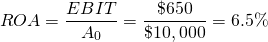
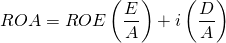
We find HQN’s rate of return on its assets, ROA, by dividing its EBIT by its beginning assets (A0) of $10,000 reported in Table 4.1 and repeated here in Table 12.2.
Table 12.2. Year End Balance
Sheets for HQN (all numbers in 000s)
Open HQN Coordinated Financial Statement in MS Excel
| BALANCE SHEET | ||
| DATE | 12/31/2017 | 12/31/2018 |
| Cash and Marketable Securities | $930 | $600 |
| Accounts Receivable | $1,640 | $1,200 |
| Inventory | $3,750 | $5,200 |
| Notes Receivable | $0 | $0 |
| Total Current Assets | $6,320 | $7,000 |
| Depreciable Assets | $2,990 | $2,710 |
| Non-depreciable Assets | $690 | $690 |
| Total Long-Term Assets | $3,680 | $2,400 |
| TOTAL ASSETS | $10,000 | $10,400 |
| Notes Payable | $1,500 | $1,270 |
| Current Portion Long-Term Debt | $500 | $450 |
| Accounts Payable | $3,000 | $4,000 |
| Accrued Liabilities | $958 | $880 |
| Total current Liabilities | $5,958 | $6,600 |
| Non-Current Long Term Debt | $2,042 | $1,985 |
| TOTAL LIABILITIES | $8,000 | $8,585 |
| Contributed Capital | $1,900 | $1,900 |
| Retained Earnings | $100 | ($85) |
| Total Equity | $2,000 | $1,815 |
| TOTAL LIABILITIES AND EQUITY | $10,000 | $10,400 |
(12.2)
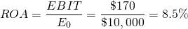
We find HQN’s ROE the rate of return on its equity by subtracting from EBIT interest costs that represent return on debt. We refer to the result as earnings before taxes (EBT). Dividing EBT by the firm’s beginning equity E0 reported in Table 12.2 as $2,000 we find:
(12.3)
AIS estimates of EBIT and EBT represent changes in the firm’s assets and equity. However, these changes in assets and equity may not be reflected by the difference between assets and equity in the beginning and ending balance sheets unless we make some adjustments. In Table 12.2, the change in equity equals $1815 – $2,000 = ($185) compared to an EBT of $170 estimated from its AIS. If we subtract from EBT taxes of $68 and owner draw of $287 we find the same difference:
(12.4)

Table 12.2 reports a change in HQN’s assets of $400 ($10,400 minus $10,000). Meanwhile HQN’s AIS reports a change in HQN’s assets, EBIT, of $650. Again part of this difference can be explained by owner draw of $287 that when added to $400 equals $687 still leaving a discrepancy of $37. In this case, the discrepancy occurs because reducing cash balances to retire some liabilities also reduces assets but not equity.
Reorganizing AIS data entries. We can reorganize AIS data into cash flow and changes in operating and capital accounts to build an IRR model that is more appropriate for analyzing multi-period investment problems. This reorganization is required because cash flow and changes in operating and capital account liquidations in IRR models may occur in several different periods while in an AIS they occur in the same period. Separating AIS entries into cash flow and changes in operating and capital accounts produces Tables 12.3 and 12.4:
Table 12.3. HQN 2018 Cash Receipts minus Cash Expenses
| Cash Receipts (CR) | ||
| + | Cash receipts from operations | $38,990 |
| + | Realized capital gains | $0 |
| = | Cash Receipts (CR) | $38,990 |
| Cash Expenses (CE) | ||
| + | Cash COGS | $27,000 |
| + | Cash OE | $11,078 |
| = | Cash Expenses (CE) | $38,078 |
| Cash Receipts – Cash Expenses = CR – CE | $912 | |
Table 12.3 divides cash flow into cash receipts (CR) and cash expenses (CE). The sources of cash receipts include cash sales from operations, realized capital gains, reductions in accounts receivable (∆AR < 0), and reductions in inventories held for sale (∆Inv < 0). The sources of cash expenses include cash payments for costs of goods sold (COGS) and cash overhead expenses (OE), reductions in accounts payable (∆AP < 0), and reductions in accrued liabilities (∆AL < 0). We measure reductions in the book value of capital assets in the tth period as depreciation (Dept). We record changes in operating and capital accounts in Table 12.4. Asset account changes include ∆AR and ∆Inv. Changes in liability accounts include ∆AP and ∆OE
Table 12.4. HQN 2018 Changes in operating accounts and depreciation
| + | Change in accounts receivable (∆AR) | ($440) |
| + | Change in inventories (∆Inv) | $1450 |
| – | Change in accounts payable (∆AP) | $1,000 |
| – | Change in accrued liabilities (∆AL) | ($78) |
| = | Changes in operating accounts | $88 |
| – | Depreciation (Dep) | $350 |
| = | Changes in capital accounts | $350 |
| = | Changes in operating and capital accounts | ($262) |
To summarize the calculations included in Tables 12.3 and 12.4 we express EBIT as:
(12.5)

Notice that the sum of cash flow recorded in Table 12.3 of $912 plus changes in operating accounts (∆AR + ∆INV – ∆AP – ∆AL – Dep) recorded in Table 12.4 of ($262) equal EBIT of $650, an amount equal to the difference in total revenue and total expenses recorded in Equation \ref{12.1}. Of course, the IRR model estimates of ROA and ROE must equal the AIS estimates of ROA and ROE since the changes in assets and equity are the same—merely rearranged entries in the two estimation methods.
Accrual Income Statements (AIS) and Internal Rate of Return (IRR) Models
EBIT and ROA
We previously calculated ROA as EBIT divided by beginning assets A0. Multiplying ROA by A0 we equate asset earnings to EBIT:
(12.6)

Now suppose that we add A0 to both sides of Equation \ref{12.6} and factor A0 on the left hand side of the equation to obtain (1 + ROA)A0. Finally, assume that we divide both sides of Equation \ref{12.5} by (1 + ROA) to obtain an IRR PV model:
(12.7)

Generally, a PV model is one that converts future values of changes in assets and equity to their present value equivalent. Consistent with that PV model definition, IRR is a PV model that discounts future assets earnings to an amount equal to its beginning assets. To avoid double counting returns and expenses in PV models, we only account for changes in operating and capital account when we convert them into cash.
To write the multi-period equivalent of Equation \ref{12.7}, we first subscript our variables for time t. To convert cash flow and liquidated values of noncash operating and capital accounts to their present value we discount them at the discount rate (1 + ROA). However, the discount rate in the multi-period equation is not the ROA derived from the one-period AIS but a multi-period average internal rate of return on assets (IRRA)that we substitute for ROA. We summarize our results in Equation \ref{12.8}:
(12.8)
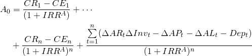
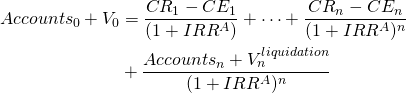
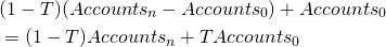
We simplify Equation \ref{12.8} by substituting ∆Accountst for ∆ARt + ∆Invt – ∆APt – ∆ALt and by recognizing the equality between beginning and ending account balances and the sum of periodic changes in accounts:
(12.9)
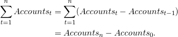
Finally, since Accounts0 and V0 equal acquisition investment cash flow and Accountsn and Vn equal liquidation investment cash flow, we enter them in the period in which they occur and rewrite Equation \ref{12.8} as Equation \ref{12.10}:
(12.10)
EBT and ROE
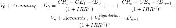
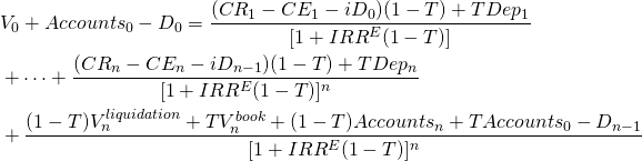
The difference between ROA and ROE is that ROA computes earnings generated by all of the firm’s assets. ROE computes only earnings produced by the firm’s equity by subtracting from total asset earnings interest earned by the firm’s liabilities. To find the multi-period IRR for equity, IRRE, we subtract in each period t interest cost iDt–1 where Dt–1 equals the firm’s debt at the end of the previous period and i equals the average cost of debt. Cash flow changes in debt are ignored since they do not represent earnings from equity. To find the amount of equity invested, we subtract from initial assets initial debt D0. Outstanding debt during the period of analysis collects interest. No changes in debt occur in the last period and debt at the end of the period n–1, Dn–1, is retired in the last period. Revising Equation \ref{12.10} to account for interest costs and debt—and replacing IRRA with the multi-period equivalent of ROE, IRRE, we can write:
(12.11)
After-tax ROA and ROE Measures
PV models mostly use after-tax cash flow (ATCF). They focus on ATCF because it represents what the firm/investors keep after paying all their expenses including taxes. In what follows we present tax obligations in a simplified form to illustrate their impact on after tax rate of return measures.
Let the average tax rate applied to equity earnings be T. Let the average tax rate applied to asset earnings be T* that depends on T. Our goal is to find the average tax rate T that adjusts ROE to ROE(1–T) and T* that adjusts ROA to ROA(1–T*). We do not try to duplicate the complicated processes followed by taxing authorities to find T and T*.
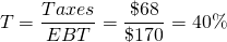
AIS report taxes paid by the firm and subtracts them from EBT to obtain net income after taxes (NIAT). We assume interest costs found by multiplying the average interest rate i times beginning period debt Dt–1 (iDt-1), have already been subtracted from earnings and used to reduce tax obligations. As a result, NIAT represents changes in equity after both interest and taxes have been paid. In 2018, HQN paid $68 in taxes. To find the average tax rate HQN paid on its changes in equity we set taxes equal to the average tax rate T times EBT:
(12.12)

Solving for the average tax rate T HQN paid on its earnings we find:
(12.13)
Finally, we adjust ROE for taxes and find HQN’s after-tax rate of return to be:
(12.14)

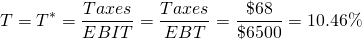
AIS Statements and After-tax ROA. AIS compute taxes paid by the firm on its returns to equity but not on its returns to assets. AIS record only one value for taxes paid and these estimates account for interest payment tax savings. As a result, the average tax rate T calculated for taxes on equity cannot be used to adjust ROA for taxes. To find the average tax rate T* that adjusts ROA to ROA(1–T*), we calculate taxes “as if” there were no interest costs to reduce the average tax rate T*. We find ROA(1–T*) in Equation \ref{12.15} as:
(12.15)

Solving for T* we find:
(12.16)

Equation (12.16) emphasizes an important point, that adjusting ROE and ROA for taxes nearly always requires different average tax rates. The only time that T = T* is when interest costs are zero. In that particular case, we can easily demonstrate that T* = T since EBIT = EBT:
(12.17)
A note on discount rates and the weighted cost of capital (WCC). It is common in many finance texts to assume that the discount rate is an exogenous variable observed in the financial markets. In small firms, the focus of this book, the discount rate depends on the rate of return earned by the defender and sacrificed to acquire the challenging investment.
The weighted average cost of capital (WACC) is the rate that a company is expected to pay on average to finance its assets. The WACC is commonly referred to as the firm’s cost of capital. Importantly, it is dictated by the external market and not by management. For small firms, we find a concept similar to the WCC that depends on the IRR of the defender and its average cost of debt. We can derive such a measure by solving for ROA in Equation \ref{8.20} that is repeated below:
(12.18)

from which we find that ROA is an equivalent measure to the WCC:
(12.19)
After-tax Multi-period IRR Models
After-tax Multi-period IRRE Model
Having found the after-tax discount rates ROE(1 – T) we are prepared to introduce taxes into multi-period IRRE PV model described in Equation \ref{12.11}. We begin by replacing IRRE with IRRE(1 – T). Then we adjust cash flow and changes in operating and capital accounts for taxes. Consider additional changes required in our IRRE PV model described in Equation \ref{12.11} to account for taxes.
Interest costs. Interest costs are returns paid for the use of borrowed money, similar to rent. Therefore, interest costs represent an expense to the firm or investment and should reduce taxable income.
Depreciation. Depreciation is a noncash event and by itself does not create a cash flow. However, it has cash flow consequences because it provides a tax shield for some income because it can be treated as an expense that reduces taxable income. Therefore ATCF must account for tax savings from depreciation equal to the average tax rate T times depreciation for the period: (T)(Dep).
Capital gains (losses) and taxes. At the
end of the analysis, PV models liquidate capital accounts for an
amount equal to  .
For tax purposes, capital assets are valued at their depreciated
book value of
.
For tax purposes, capital assets are valued at their depreciated
book value of  .
If the difference between the liquidation and book value of capital
assets is positive,
.
If the difference between the liquidation and book value of capital
assets is positive,  0," title="Rendered by QuickLaTeX.com" height="22" width="195"
style="vertical-align: -4px;"> the firm or the investment has
earned capital gains or depreciation recapture whose after-tax
value is
0," title="Rendered by QuickLaTeX.com" height="22" width="195"
style="vertical-align: -4px;"> the firm or the investment has
earned capital gains or depreciation recapture whose after-tax
value is  0." title="Rendered by QuickLaTeX.com" height="22" width="252"
style="vertical-align: -4px;"> On the other hand, if the
difference is negative
0." title="Rendered by QuickLaTeX.com" height="22" width="252"
style="vertical-align: -4px;"> On the other hand, if the
difference is negative  then the firm has suffered a capital loss and earned tax credits.
In the case of capital losses, the difference that represents a
loss in value to the firm is reduced to
then the firm has suffered a capital loss and earned tax credits.
In the case of capital losses, the difference that represents a
loss in value to the firm is reduced to  Finally, to adjust capital accounts for taxes, we add the original
book value .
We summarize these results below:
Finally, to adjust capital accounts for taxes, we add the original
book value .
We summarize these results below:
(12.20)
We make similar adjustments to the firm’s operating account balances. We adjust changes in account balances for tax consequences. Letting the liquidation value of accounts equal Accountsn and the acquisition value of accounts equal to Accounts0, we write the after-tax liquidation value of accounts as:
(12.21)
Now we can write the after-tax IRRE model for changes in equity consistent with principles followed when we constructed one-period AIS as:
(12.22)
After-tax Multi-period IRRA Model
There is a paradox in applied PV models. The paradox is that there is no explicit measure for T* that can be used to find ROA(1 – T*). This peculiar result occurs because taxes must account for interest costs that are not considered in EBIT measures. Yet, most applied IRR models solve for after-tax return on assets that should be guided by ROA(1 – T*) calculations.
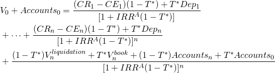
To properly account for taxes when finding in an IRRA model we should apply the tax rate T* to earnings on assets. Adjusting (12.20) by eliminating interest costs while allowing them to influence taxes paid and replacing IRRE with IRRA, we can express the after-tax multi-period IRRA model as:
(12.23)
Consistency and IRRA(1 – T*) and IRRE(1 – T) PV model rankings
We can construct PV models that find either before or after-tax returns on equity or assets and use them to rank investments. Furthermore, the IRRA(1 – T*) and IRRE(1 – T) rankings need not be consistent with IRRA and IRRE rankings. One reason they need not be consistent is that their initial and periodic sizes are different (see Chapter 9). Furthermore, interest costs included in the IRRE model and not in the IRRA model allow for ranking variations
So, how do we decide on our ranking criterion? Do we focus on equity or asset earnings? Equity or asset earnings before or after-taxes are paid? Although there may not be any one satisfactory answer to this question, it surely must depend on, among other things, on what questions the financial manager wants to answer.
Net Present Value Models
The homogeneous measures principle requires that cash flow and changes in accounts for defenders and challengers be measured in consistent units. Both must be measured in either before or after-taxes. Both must be measured in return to assets or equity. Both must be measured in real or current dollars. Both must be similar in investment sizes. Both must reflect similar terms. And both should be adjusted to similar risk classes.
The homogeneous measure requirements guarantee that if two investments are compared using their IRRs or NPVs—they will be ranked the same. Furthermore, satisfying homogeneity requirements also guarantee the usual number system properties apply. In particular, if investment A is preferred to B and B is preferred to C, then A is preferred to C.
While any particular NPV model that satisfies homogeneity requirements will rank investments A and B consistently, it is not true that NPV and IRR models will produce the same rankings when homogeneity conditions change. Earlier we showed that rankings depended on which size adjustment method we adopted for rationalizing investment size differences. Now we show that rankings depend not only on what size adjustment method we adopt but also by what homogeneity conditions we adopted. For example, we can easily demonstrate that equity derived IRRs and NPVs may produce different rankings than asset derived IRRs and NPVs.
To make clear that equity versus asset derived IRR and NPV measures may produce different rankings, consider HQN’s one-period IRRA of 6.5% ($650/$10,000) and its one-period IRRE of 8.5% ($170/$2,000) respectively. Let the original HQN asset and earning measures describe investment A. Now without changing beginning assets or equity, suppose a different investment B incurred no interest costs. Then investment B’s ROA would be unchanged ($650/$10,000); however, its ROE would increase to 32.5% ($650/$2,000). Meanwhile the investor would continue to be indifferent between investments A and B based on their IRRAs (and NPVs) since both equal 6.5%. However, clearly investment B is preferred to A based on their IRREs (and NPVs).
PV Model Templates
PV models answer practical questions about investments whose costs and benefits extend over time. They can be descriptive such as IRR models that provide information about an investment’s rate of return. Or, they can be prescriptive such as NPV models that compare defender’s rate of return with a challenger’s cash flow.
To facilitate the calculation of IRRs and NPVs and to emphasize the decision maker’s important role in providing accurate and consistent data, we provide two PV model templates that correspond to equations (12.22) for equity and (12.23) for assets. In each template we calculate before and after-tax NPVs, their respective IRRs, and annuity equivalents (AE). Finally, we note that we can use the PV templates to solve one-period problems producing results equivalent to those produced by AIS. More typically, we can use them to solve multi-period problems. Finally, while we can use PV models to describe and rank the firm’s financial performance, it is more common to use PV models to describe and rank investments.
We illustrate the two templates by using HQN 2018 data. In effect, we calculate one-period NPV, AE, and IRR estimates that correspond to AIS estimates. In Chapter 13 we apply the model to describe multi-period investments.
Before-tax PV Asset Models and EBIT
We now introduce a template for assets described in Table 12.5 using HQN data for 2018 described in Tables 12.1 and 12.2. By setting T* equal to zero, the template corresponds to EBIT calculations in Table 12.1. We describe the template in Table 12.5 that follows.
Table 12.5. PV Template for
Rolling NPVs, AEs, and IRRs Earned by Assets Before Taxes are
Paid.
Open Table 12.5 in Microsoft Excel
| A | B | C | D | E | F | G | H | I | J | K | L | M | N | O | P | |
| 3 | Yr | Capital accounts values | Capital accounts liquidation value | Capital accounts book value | Operating accounts values (AR- INV – AP – AL) | Capital Accounts Depr. | Cash Receipts (CR) | Cash Cost of Goods Sold (COGS) | Cash Overhead Expenses (OEs) | The savings from depr. (TxDepr) | After-tax cash flow (ATCF) from operations | ATCF from liquidating Capital and operating accounts | ATCF from operations and liquidations | Rolling NPVs | Rolling AEs | Rolling IRRS |
| 4 | 0 | $8,558 | $8,558 | $1,442 | ||||||||||||
| 5 | 1 | $0 | $8,218 | $8,208 | $1,520 | $350 | $38,990 | $27,000 | $11,078 | $0 | $912.00 | $9,738.00 | $10,650 | $0.00 | $0.00 | 6.50% |
The column headings in Table 12.5 describe exogenous and endogenous variables used to find rolling (every year) NPV, AE, and IRR estimates.
- Column A lists the periods at the end of which financial activity occurs.
- Column B lists capital investment amounts.
- Column C lists the liquidation value of capital investments.
- Column D lists the book value of capital investments.
- Column E lists the value of operating accounts at the end of each period (AR + Inv – AP – AL).
- Column F calculates depreciation equal to the change in the investment’s book value determined by tax regulations.
- Column G reports CR equal to the sum of cash sales plus negative changes in AR and Inv.
- Column H reports cash COGS equal to cash operating expenses plus reductions in AP.
- Column I reports cash OE equal to cash overhead expenses plus reductions in AL.
- Column J calculates tax saving created by depreciation, relevant only in after-tax models.
- Column K calculates cash flow from operations equal to CR less cash COGS and cash OE.
- Column L calculates cash flow from liquidation of capital assets and operating accounts.
- Column M sums cash flow from operations and liquidations.
- Column N calculates rolling NPVs as though the investment ended in each year.
- Column O calculates rolling AEs associated with the NPV for each year.
- Finally, column P finds rolling IRRs for each investment life.
Note that operating cash flow equal to $912 (Column K) correspond to the sum of operating cash flow in Table 12.3 and is found by adding cash receipts (Column G) less cash COGS (Column H) and cash OE (Column I). We report the total liquidation value in column L as an amount equal to the investment’s liquidation value reported in column C plus the change in the sum of accounts in successive years reported in Column E. The sum of operating cash flow reported in column K plus the liquidation value of operating and capital accounts reported in Column L equals the value of the firm reported in Column M. Finally, the change in assets equals the value reported in Column M less the beginning value of assets reported in cell B4 equals $650 corresponding the HQN’s EBIT value reported in Table 12.1. It follows that EBIT divided by assets of $10,000 is the one-period ROA calculated from the AIS and the one-period IRRA calculated in the PV template reported in Table 12.5, both equal to 6.5%. Furthermore, if we discount the ending value of the firm by its IRR, its NPV is zero as is its AE since the discount rate used in cell N4 is the IRR.
Change in operating accounts. Table 12.5 is intended to model Equation \ref{12.21}. And for the most part, the similarities are transparent. The initial investment that includes operating accounts and capital assets equals total assets of $10,000. The change in the capital accounts equals depreciation of $350. Cash flow during the period is cash receipts less cash expenses equal to $912 is easy to associate with Equation \ref{12.21}. However, the change in operating accounts need some explanation.
Beginning (ending) operating accounts are calculated from HQN’s beginning (ending) balance sheet. Beginning assets less beginning operating account balances equal beginning capital account value. Beginning capital account balances less depreciation equals ending book value for capital account balances.
Before-tax PV Equity Models and EBT
We now introduce a PV template for equity described in Table 12.6 that corresponds to equation 12.20. We populate the template using HQN data for 2018 described in Tables 12.1 and 12.2. By setting the tax rate T equal to zero, the results corresponds to EBT calculations in Table 12.1.
Table 12.6. PV Template for
Rolling Estimates of NPVs, AEs, and IRRs for Equity Earnings Before
Taxes
Open Table 12.6 in Microsoft Excel
| A | B | C | D | E | F | G | H | I | J | K | L | M | N | O | P | Q | R | |
| 3 | Yr | Capital accounts values | Debt Capital | Capital accounts liquidation value | Capital accounts book value | Operating accounts values (AR- INV – AP – AL) | Capital Accounts Depr. | Cash Receipts (CR) | Cash Cost of Goods Sold (COGS) | Cash Overhead Expenses (OEs) | Interests Costs | The savings from depr. (TxDepr) | After-tax cash flow (ATCF) from operations | ATCF from liquidating Capital and operating accounts | ATCF from operations and liquidations | Rolling NPVs | Rolling AEs | Rolling IRRS |
| 4 | 0 | $8,558 | $8,000 | $8,558 | $1,442 | |||||||||||||
| 5 | 1 | $0 | $8,080 | $8,208 | $8,208 | $1,530 | $350 | $38,990 | $27,000 | $11,078 | $480 | $0 | $432.00 | $1,738 | $2,170 | $0.00 | $0.00 | 8.50% |
| 6 | 2 | $0 | $8,000 | $20,000 | $20,000 | $1,200 | -$6,792 | $29,800 | $13,500 | $11,189 | $485 | $0 | $4,626.42 | $13,120 | $17,746 | $15,472.9 | $7,336.47 | 0.00% |
The column headings in Table 12.6 are only slightly modified from those reported in Table 12.5.
- Column A lists the periods at the end of which financial activity occurs.
- Column B lists investment (equity) amounts for which NPVs, AEs, and IRRs are calculated.
- Column C lists the debt and other liabilities supporting the investment.
- Column D lists the liquidation value of the investment (equity).
- Column E lists the book value of investments.
- Column F lists the net value of operating accounts at the end of each period (AR + Inv – AP – AL).
- Column G calculates depreciation equal to the change in the investment’s book value determined by tax regulations.
- Column H reports cash receipts equal to the sum of cash sales plus negative changes in AR and Inv.
- Column I reports cash COGS equal to cash operating expenses plus reductions in AL.
- Column J reports cash OE equal to cash overhead expenses plus reductions in the AL account.
- Column K reports interest paid on debt and other liabilities.
- Column L calculates the tax saving created by depreciation, relevant only in after-tax models.
- Column M calculates cash flow from operations.
- Column N calculates cash flow from liquidation.
- Column O sums cash flow from operations and liquidation.
- Column P calculates NPV as though the investment ended in each year.
- Column Q calculates the AE associated with the NPV for each year.
- Finally, column R finds the IRR for each investment life.
Note that operating cash flow of $432 (Column M) corresponds to the sum of operating cash flow in Table 12.3 and is found by adding cash receipts (Column H) less cash COGS (Column I), cash OE (Column J) and interest costs (Column K). The equity liquidation value of the investment is reported in column D. The book value of the investment is listed in column E. The total liquidation value less debt and liabilities outstanding at the end of the previous period are reported in Column N. The sum of operating cash flow plus the liquidation value of operating and capital accounts less outstanding debt are reported in Column O . Finally, the change in equity equals the value reported in cell O5 less the value reported in cell O4, an amount equal to $170 corresponding to HQN’s EBT in Table 1. It follows that EBT divided by equity of $2000 is the one-period ROE and the one-period IRRE, both equal to 8.5%. Furthermore, if we discount the ending value of the firm by its IRR reported in cell P4, its NPV is zero as is its AE since the discount rate is its IRR.
Change in operating accounts. Table 12.6 is intended to model Equation \ref{12.21} and for the most part, the similarities are transparent. The initial investment that includes accounts and capital assets less initial debt is the same and equal to $2,000. The change in the capital accounts is equal to depreciation and the difference between beginning and ending capital accounts of $350. The cash flow during the period of cash receipts less cash expenses equal to $912 less interest costs of $480 are also easy to connect. However, the change in operating accounts need some explanation.
Beginning operating accounts are included in the beginning investment (assets). They are also included in the book value of the investment unchanged from the beginning investment amount. To include changes in operating account to adjust beginning investment to liquidated investment value, we add the difference between the operating accounts at the beginning and ending period.
After-tax PV Equity Models and NIAT
AIS introduce taxes into its return on equity calculations by subtracting taxes paid from EBT (see Table 12.1). The result is net income (earned on equity) after taxes, NIAT. We introduce taxes into Table 12.6 by adjusting cash to an after-tax basis by multiplying operating cash flow less interest costs by (1 – T) where T was found earlier to equal to T = .4. The after-tax cash flow from operations, operating ATCF, we report in column M. In addition, we must account for tax savings generated by depreciation reported in column L. Finally, tax consequences from any capital gains (losses) adjust liquidation cash flow reported in column N. The template corresponding to NIAT and after-tax return to equity we report in Table 12.7.
Table 12.7. PV Template for
Rolling Estimates of NPVs, AEs, and IRRs for Equity Earnings After
Taxes
Open Table 12.7 in Microsoft Excel
| A | B | C | D | E | F | G | H | I | J | K | L | M | N | O | P | Q | R | |
| 3 | Yr | Capital accounts values | Debt Capital | Capital accounts liquidation value | Capital accounts book value | Operating accounts values (AR- INV – AP – AL) | Capital Accounts Depr. | Cash Receipts (CR) | Cash Cost of Goods Sold (COGS) | Cash Overhead Expenses (OEs) | Interests Costs | The savings from depr. (TxDepr) | After-tax cash flow (ATCF) from operations | ATCF from liquidating Capital and operating accounts | ATCF from operations and liquidations | Rolling NPVs | Rolling AEs | Rolling IRRS |
| 4 | 0 | $8,558 | $8,000 | $8,558 | $1,442 | |||||||||||||
| 5 | 1 | $0 | $8,080 | $8,208 | $8,208 | $1,520 | $350 | $38,990 | $27,000 | $11,078 | $480 | $140 | $399.20 | $1,702.80 | $2,102 | $0.00 | $0.00 | 5.10% |
Note that in column O, the difference between the beginning and ending equity is $102, the same value reported for NIAT in Table 12.1. Furthermore, dividing $102 by the beginning equity of the firm produce an after-tax ROA and an after-tax IRRE(1 – T) of 5.1%. Finally, if we change the discount rate in cell P4 we find NPV and AE are equal to zero since the discount rate is also the after-tax IRR.
Summary and Conclusions
We now make explicit the main point of this chapter. PV models are multi-period expressions of information found in single-period AIS. IRRA and IRRE derived in IRR models correspond to ROA and ROE measures derived from single-period AIS. Furthermore, EBIT measures calculated in AIS models correspond to earnings from assets in PV models. EBT corresponds to earnings from equity in PV models, and NIAT corresponds to after-tax earnings from equity in PV models. While there is no explicit AIS measure of after-tax earnings from assets, it can be implied and easily measured.
Rates of return measures derived in AIS and IRR models are descriptive in nature—they describe a single investment. However, we can use also use them prescriptively by comparing them with IRRs of other firms and investments. However, we can construct a prescriptive PV model, an NPV model, by discounting cash flow from a challenging investment using the IRR of a defending investment. (The challenging investment is one considered for a replacing to a defending investment already in use by the firm.). If the NPV is positive (negative), we recommend replacing (leaving in place) the defending investment.
There are other PV models besides IRR and NPV models. We described these in Chapter 8. Most other PV models are variants of the NPV or IRR model. Maximum bid (minimum sell) models find the maximum bid (minimum sell) that can be paid (received) for a challenger and still earn the IRR of the defender. Loan formulae are special PV models that describe the amount that must be paid to receive a challenging loan while the defending loan earns its interest rate. AE simply find a multi-period time adjusted average of a challenger’s cash flow. Replacement flows are special NPV models that find the optimal life of a repeatable investment that maximizes its NPV and the NPV of future replacements.
The next step in our study of PV models is to generalize them to multi-periods and use them to solve practical investment problems. Both of these tasks, we undertake in chapter, Chapter 13.
Questions
- List similarities and differences between an AIS statement and a PV model.
- Both AIS and PV models find rates of return on assets and equity using cash flow and changes in operating and capital asset accounts. However, they organize them differently. Explain how AIS and PV models organize cash flow and changes in operating and capital asset accounts differently.
- We can describe ROA and ROE as measures of changes in assets and equity respectively divided by original asset and equity values. Please explain.
- EBIT measures the change in the value of the firm’s assets before adjusting for taxes during a single period. Do you agree or disagree? Defend your answer.
- EBT measures the change in the value of the firm’s equity before adjust for taxes during a single period. Do you agree or disagree? Defend your answer.
- Measures the change in the value of the firm’s equity after adjusting for taxes during a single period. Do you agree or disagree? Defend your answer.
- There is no measure in an AIS statement that finds the change in assets after adjusting for taxes. Can you explain why?
- Use the template reported in Table 12.5 to find the change in assets after adjust for taxes. To find the after-tax change in assets, use an average tax rate of T*=10.46% and a discount rate of ROA(1 – T*) = (6.5%)(1 – 10.46%) = 5.8%.
- Describe the conditions under which NPV or IRR asset and equity models would rank challenging and defending investment consistently.
- Give an example in which NPV or IRR asset and equity models rank challenging and defending investments inconsistently.
- As a financial manager tasked with ranking a defending and a challenging investment, which ranking criteria would you employ: NPV earned by equity or NPV earned by assets? Defend your answer.