
9: Homogeneous Sizes
- Page ID
- 12754

At the end of this chapter, you should be able to: (1) understand how internal rate of return (IRR) and net present value (NPV) models can produce inconsistent rankings; (2) produce consistent IRR and NPV rankings by adjusting for investment size differences and by adopting common reinvestment rate assumptions; (3) understand why some NPV and IRR rankings are unstable; (4) recognize how different initial size adjustment methods (addition, scaling, or some combination) produce consistent but sometimes different investment rankings; and (5) recognize how investment type differences can be used to identify the proper size adjustment method.
To achieve your learning goals, you should complete the following objectives:
- Recognize that IRR and NPV rankings may be inconsistent and that NPV rankings may be unstable.
- Understand the difference between periodic investment sizes and initial investment sizes.
- Describe how different reinvestment rate assumptions can produce inconsistent IRR and NPV rankings.
- Show how resolving periodic and initial size differences and a common reinvestment rate produce consistent challenging investment rankings.
- Illustrate the different methods available for resolving periodic size investment differences.
- Demonstrate how scaling and addition can be used to resolve initial size differences in investments.
- Demonstrate that while different methods for resolving periodic and initial size differences can each produce consistent rankings, the consistent rankings may not be the same.
- Understand the conditions under which IRR and NPV provide the same rankings as the size adjusted IRR and NPV models.
- Recognize the four basic investment models
- Recommend the appropriate investment model based on challenger characteristics.
Introduction[1]
In the single equation NPV model, we assumed that cash flow was exchanged between time periods at the defender’s IRR. In the single equation IRR model, we assumed that cash flow was exchanged between time periods at the challenger’s IRR. In the NPV model, the challenger (defender) was preferred to the defender (challenger) if the NPV were positive (negative). Furthermore, the NPV ranking of the defender and challenger was the same ranking obtained by comparing their respective IRRs. As a result, both IRR and NPV criteria produce the same ranking.
This chapter recognizes that when we rank multiple challengers funded by one defender, their IRR and NPV rankings may be different. Furthermore, we observe that changes in the defender’s IRR may produce unstable NPV rankings. We demonstrate these results in Table 9.1 that ranks three challengers.
initial investments
 where i = 1,2,3
 |
period one cash flows
 where
t = 1 generated by initial investments
where i = 1,2,3 where
t = 1 generated by initial investments
where i = 1,2,3 |
period two cash flows
where
t = 2 generated by initial investments
where i = 1,2,3 |
NPVi earned by
initial investments
where i = 1,2,3 assuming r = 5% (ranking) |
NPVi earned by
initial investments
where i = 1,2,3 assuming r = 10% (ranking) |
IRRi earned by
initial investments
where i = 1,2,3 (ranking) |
|---|---|---|---|---|---|
| $1,000 | $800 | $400 | $124.72 (3) |
$57.85 (2) |
14.8% (1) |
| $2,000 | $1,560 | $800 | $211.34 (2) |
$79.34 (1) |
13.3% (2) |
| $3,000 | $2,250 | $1,200 | $231.29 (1) |
$37.10 (3) |
11.0% (3) |
We describe the challenging investments’ NPV rankings in columns 4 and 5 for investments of $1,000, $2,000, and $3,000. The investments’ IRR rankings appear in column 6. We indicate investment rankings by parenthesized numbers in columns 4, 5, and 6.
If the defender’s IRR is 5% for challenging investments 1, 2, and 3, their NPV rankings are 3, 2, and 1 respectively. If the defender’s IRR is 10% for challenging investments 1, 2, and 3, their NPV rankings are 2, 1, and 3 respectively. Meanwhile, for challenging investments 1, 2, and 3 their IRR rankings are different still: 1, 2, and 3 respectively. These results demonstrate that IRR and NPV rankings may provide inconsistent rankings and NPV rankings may vary with the defender’s IRR.
The inconsistent IRR and NPV rankings require decision makers to choose between conflicting recommendations. They must decide: which ranking method should they believe. Among practitioners, the NPV approach is considered more reliable for wealth maximization. However, the ease in which decision makers can interpret IRRs has made it the more popular of the two ranking methods. Both ranking methods, however, have their drawbacks. Investments may have multiple IRRs and NPV rankings may be unstable—varying with changes in the defender’s IRR what is often referred to as the discount rate.
The problem produced by inconsistent IRR and NPV rankings is obvious—it leaves decision makers without a clear recommendation. On the other hand, NPV rankings that vary with the discount rate (see columns four and five) can be just as problematic. The reason is that if we are not sure of the discount rate, then we cannot be sure of the NPV rankings either.
The purpose of this chapter is to demonstrate that by resolving periodic and initial investment size differences between challenging investments and by adopting a common reinvestment rate, we can guarantee consistent IRR and NPV rankings. We will also explain why some NPV rankings vary with changes in the defender’s IRR. Finally, we show that depending on how we adjust for size differences and the reinvestment rate we adopt, we an produce four different present value (PV) models. We also discuss the conditions under which each investment model is appropriate for ranking challenging investments—rankings that will be consistent but possibly different across models.
Periodic and Initial Investment Sizes
Sometimes when IRR and NPV methods produce inconsistent rankings, it is because the challenging investments being ranked lack investment size homogeneity. Challenging investments may lack investment size homogeneity in two ways. First, their initial investment sizes may be different. In Table 9.1 note that challenging investments 1, 2, and 3 invested initial amounts of $1,000, $2,000, and $3,000 respectively.
The second way challenging investment sizes may differ is their periodic cash flows. These differences change periodic investment amounts between challenging investments. Notice that in Table 9.1 cash flows in period one are different: $800, $1,560, and $2,250 for investments 1, 2, and 3 respectively. Differences in initial and periodic investment sizes contribute directly to inconsistent and unstable rankings.
Notation. This chapter employs more than
the usual amount of mathematical notation. It is required to tell
the story about consistent and stable IRR and NPV rankings. The
good news is that there are no complicated mathematical operations
besides adding, subtracting, canceling like terms, and factoring.
The notation that will be used throughout this chapter includes
variables with subscripts and superscripts. The superscript on a
variable associates it with an investment, i = 1, 2, …,
m. The subscript on a variable associates it with a time
period t = 1, …, n. If a superscripted variable
is raised to a power, the variable is placed in parentheses and the
power to which the variable is raised is placed outside of the
parentheses. To illustrate, the variable  describes the value for the variable R associated with
investment i = 2 in the t = 5 time period raised
to the third power. Finally, when we write an expression like
describes the value for the variable R associated with
investment i = 2 in the t = 5 time period raised
to the third power. Finally, when we write an expression like
 we are saying that function S depends on values assumed by
variables r and
without specifying the exact nature of the function or the values
of the variables represented by r and .
When we want to represent a vector of values for investment
i we bold R and write
we are saying that function S depends on values assumed by
variables r and
without specifying the exact nature of the function or the values
of the variables represented by r and .
When we want to represent a vector of values for investment
i we bold R and write 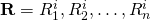 .
.
How differences in periodic cash flow can
create periodic investment size differences. Applying the
notation described earlier, we now demonstrate how differences in
cash flow create differences in investments sizes over time. Assume
that initial investments of
for investments i = 1 and i = 2 equal
V0. Also assume that cash flows in period one
earned by investments one and two are equal to  and
and  respectively. These positive (negative) cash flows represent
investments (disinvestments) in the underlying investment. If the
initial investments earned a rate of return equal to the defender’s
IRR equal to r, then beginning in period two, investment
one equals
respectively. These positive (negative) cash flows represent
investments (disinvestments) in the underlying investment. If the
initial investments earned a rate of return equal to the defender’s
IRR equal to r, then beginning in period two, investment
one equals 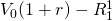 and investment two equals
 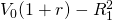 which are not equal if
  .
As a result, unequal periodic cash flows create unequal periodic
investments, even if their initial investments are equal, a cause
of inconsistent rankings.
.
As a result, unequal periodic cash flows create unequal periodic
investments, even if their initial investments are equal, a cause
of inconsistent rankings.
To illustrate numerically, suppose that
V0 = $100 and  and
and  .
If r is 10% then after one period the amount invested in investment
one is $100(1.1) – $15 = $95 and the amount invested after one
period in investment two is $100(1.1) – $20 = $90. After one period
the investment amounts are unequal and violate the homogeneity of
measures requirement.
.
If r is 10% then after one period the amount invested in investment
one is $100(1.1) – $15 = $95 and the amount invested after one
period in investment two is $100(1.1) – $20 = $90. After one period
the investment amounts are unequal and violate the homogeneity of
measures requirement.
The implication of these results is that even though two investments begin with equal initial investments, IRR and NPV rankings may still be inconsistent and unstable if periodic cash flows are unequal.
So what have we learned? We’ve learned that the two homogeneous investments size conditions required for consistent NPV and IRR rankings are 1) equal initial challenging investments sizes, and 2) equal periodic cash flows except in the last period. We require equal periodic cash flows except in the last period to ensure that the challenging investments will satisfy equal periodic investment sizes. Besides these two size conditions, one of two reinvestment rate assumptions must be adopted for both NPV and IRR rankings. These two reinvestment rate assumption are that cash flow are either reinvested at the defender’s IRR or at the challengers’ respective IRRs.
Consistent IRR and NPV Rankings When the Reinvestment Rate is the Defender’s IRR
To be clear, reinvestment rates indicate where periodic cash flows will be reinvested. If the reinvestment rate is the defender’s IRR, then we assume that earnings from the challenging investments will be reinvested in the defender. If the reinvestment rates are the challenging investments’ respective IRRs, then we assume that earnings from the investments will be reinvested in the challenging investments. If there is some other reinvestment rate, it must correspond to a separate investment and be evaluated as another challenger. Hence, the only reinvestment rates we consider are the defender’s IRR and the challenging investments’ IRRs.
NPV models implicitly assume that the reinvestment rate is the defender’s IRR and earnings from the investment will be reinvested in the defender. IRR models assume that the reinvestment rate is the investment’s own IRR and that the funds will be reinvested in itself. However, to remove ranking inconsistencies, we impose the same reinvestment rate across IRR and NPV models and produce what others have referred to as modified IRR (MIRR) and modified NPV (MNPV) models.
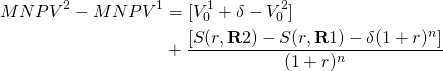
Next we demonstrate that if the two sufficient size conditions are satisfied and challenger earnings are reinvested in the defender, we are guaranteed consistent NPV and IRR rankings. NPV rankings will be consistent and under some conditions stable.
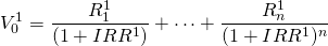
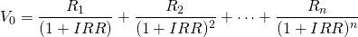
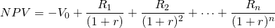
NPV rankings. Consider ranking two mutually exclusive n period investments in a similar risk class by their respective NPVs. The NPV model for investment one is described as:
\[\label{9.1a} N P V^{1}=-V_{0}^{1}+\frac{R_{1}^{1}}{(1+r)}+\cdots+\frac{R_{n}^{1}}{(1+r)^{n}}\]
The NPV model for investment two is described as:
\[\label{9.1b} N P V^{2}=-V_{0}^{2}+\frac{R_{1}^{2}}{(1+r)}+\cdots+\frac{R_{n}^{2}}{(1+r)^{n}}\]
In the equations above, r is the
defender’s IRR,  and
and  are initial investments one and two respectively, and Rt1
and Rt2 are periodic cash flows in periods t = 1,
⋯, n generated by mutually exclusive investments one and
two. We assume that the terms of the two investments are equal.
are initial investments one and two respectively, and Rt1
and Rt2 are periodic cash flows in periods t = 1,
⋯, n generated by mutually exclusive investments one and
two. We assume that the terms of the two investments are equal.
To resolve size differences caused by differences in periodic cash flows, we set them equal to zero in every period except the last one by reinvesting them at rate r until the last period. Generally, the discount rate and the reinvestment rate in NPV models are equal. To distinguish the original NPV model with the NPV model with funds reinvested until the last period, many finance scholars refer to the later model as the modified NPV model or the MNPV model. We write the MNPV model as:
(9.2a)
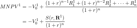
where  Similarly the MNPV model for investment two can be rewritten
as:
Similarly the MNPV model for investment two can be rewritten
as:
(9.2b)
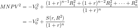
where  Finally, we impose the additional condition that
 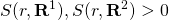 0" title="Rendered by QuickLaTeX.com" height="20" width="169"
style="vertical-align: -4px;">, otherwise the investment
decision is no longer interesting.
0" title="Rendered by QuickLaTeX.com" height="20" width="169"
style="vertical-align: -4px;">, otherwise the investment
decision is no longer interesting.
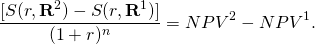
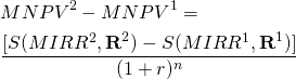
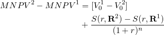
The difference between MNPV1 and MNPV2 which ranks the two investments can be expressed as:
(9.3)

If the initial investment sizes are the same as required by the homogeneity of measures principle, then the difference in the first bracketed expression in Equation \ref{9.3} is zero and the rankings will depend only on the difference between the sums of reinvested cash flows:
(9.4)
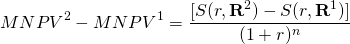
Equation (9.4) provides an interesting result. We obtained these results by reinvesting and discounting cash flow at the same rate so NPVs of the two investments are unaffected allowing us to write:
(9.5)
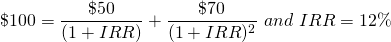
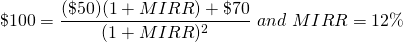
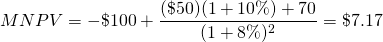
We now illustrate the results of Equation \ref{9.5}. Let the initial investment equal $100 and cash flows in periods one and two equal $50 and $70 respectively. Finally let the discount rate and the implied reinvestment rate equal 10%. Then we write:
(9.6a)
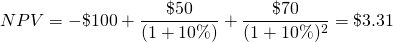
Then we write the equivalent MNPV model as:
(9.6b)
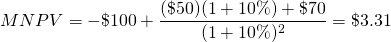
The results illustrate NPV and MNPV models are equal and provide the same rankings when the reinvestment rate is the same as the discount rate.
Finally, it should be noted that the difference between the NPVs in Equation \ref{9.5} may be unstable and change as the defender’s IRR changes as we demonstrated in Table 9.1.
IRR rankings. Consider ranking two mutually exclusive n period investments in a similar risk class by their respective IRRs. If the IRR rankings are to be consistent with the NPV rankings, they must satisfy the sufficient conditions described earlier, including assuming the same reinvestment rate r. The IRR model for investment one is described as:
(9.7a)
The IRR model for investment two is described as:
(9.7b)

In the equations above, V01 and V02 are initial
investments one and two respectively, and  and
and  are periodic cash flows in periods t = 1, ⋯, n
generated by mutually exclusive investments one and two.
are periodic cash flows in periods t = 1, ⋯, n
generated by mutually exclusive investments one and two.
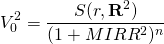
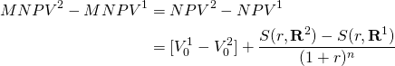
To resolve differences in periodic cash flows, we set them equal to zero in every period except the last period by reinvesting them at rate r until the last period. Generally, the discount rate and the reinvestment rate in IRR models are equal. Here, the reinvestment rate is r rather than their respective IRRs. To distinguish the original IRR model from the IRR model with funds reinvested until the last period, many finance scholars refer to the later model as the modified IRR model, the MIRR model. We write the MIRR model as:
\[\label{9.8} V_{0}^{1}=\frac{S\left(r, \mathbf{R}^{1}\right)}{\left(1+M I R R^{1}\right)^{n}}\]
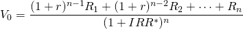
Solving for MIRR1 in Equation \ref{9.8} we obtain:
(9.9)

which has one positive root.
Investment two is described as:
(9.10)
Solving for MIRR2 in Equation \ref{9.9} we obtain:
(9.11)

which has one positive root.
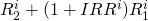
Finally, we write the difference between
MIRR1 and MIRR2 assuming initial investments
and
are equal to V0 as:
(9.12)

If the initial sizes and terms of investments one
and two are equal, then their MIRR ranking will depend on the same
criterion that ranked the investments’ MNPVs—the difference in the
sum of their reinvested cash flows  and
and  and the MIRR rankings and MNPV rankings will be consistent.
However, we cannot be certain that the MIRR rankings will equal the
IRR rankings because we changed the reinvestment rate assumption in
the IRR models.
and the MIRR rankings and MNPV rankings will be consistent.
However, we cannot be certain that the MIRR rankings will equal the
IRR rankings because we changed the reinvestment rate assumption in
the IRR models.
Consistent IRR and NPV Rankings Assuming Reinvestment Rates are the Challenging Investments’ IRRs
In this section, we demonstrate that we can also guarantee consistent NPV and IRR rankings by imposing the second reinvestment rate assumption—that periodic cash flows are reinvested in the challenging investments’ IRRs.
Suppose the reinvestment rates were the IRRs of the challengers being evaluated. This reinvestment rate is appropriate under the condition that the cash flows are reinvested in the challengers as opposed to being reinvested in the defending investment. To demonstrate the consequences of assuming that the reinvestment rates equal the challengers’ IRRs, consider the following.
Assume that the initial sizes of the challenging investments are equal and that their cash flows are reinvested in themselves earning their respective IRRs and the discount rate applied to the NPVs is the defender’s IRR. Then we could write the difference between MNPVs as:
(9.13a)
Meanwhile, we can write the difference between MIRRs as:
(9.13b)

Notice that the MNPV and MIRR rankings depend on the same sums making their rankings consistent. However, in contrast to the NPV model, the MNPV rankings are stable and likely different that the original NPV rankings. But there is one thing more. Look at the original IRR equations. They are equivalent to the MIRR equations. Reinvesting and discounting by the challengers’ IRRs are offsetting operations and don’t change the original IRRs. Therefore, if the initial sizes are equal, and the assumption is that cash flows are reinvested in the challenging investments, then IRR and MIRR rankings are equivalent! This is such an important point, we illustrate it with an example.
Assume net cash flows of $50 and $70 in periods one and two respectively, an initial investment of $100, and a reinvestment rate of the investment’s IRR or MIRR. Then we can write the IRR as:
(9.14a)
Now we can write the MIRR model as:
(9.14b)
Because the IRR and MIRR values are the same, they will return identical rankings. To emphasize the main point, if the periodic cash flows are reinvested in the challengers, then ranking investments using the investments’ IRR is the same as ranking them with their MIRRs.
So what have we learned? We learned that when we satisfy the two sufficient size conditions required for consistent rankings, equal initial and period investment sizes (except in the last period), and satisfy the second reinvestment rate assumption that we reinvest in the challenging investments—then MNPV and MIRR rankings of the challengers will be consistent. And there is one thing more, the MIRR rankings will be the same as the original IRR rankings.
We have also learned that inconsistent challenging investments IRR and NPV rankings are often the results of the two ranking methods adopting different reinvestment rate assumptions. NPV models assume the reinvestment rate is the defender’s IRR. IRR models assume the reinvestment rate is the challenger’s IRR for the same investment. Consistency requires that the reinvestment rate for each investment be the same regardless of whether the ranking tool is IRR or NPV. Once we have satisfied initial and periodic investment size differences and adopted a consistent reinvestment rate assumption, investments can be ranked consistently using IRR or NPV methods.
Reinvestment rates and inconsistent rankings. To make clear that consistent IRR and NPV rankings require that the same reinvestment rate for each investment regardless of the ranking methods, IRR or NPV, we describe three investments with the same initial sizes and assume the defender’s IRR is 5%. We allow NPV models to reinvest at the defender’s IRR rate of 5%. We allow the challenger’s cash flow to be reinvested at their respective IRRs. The inconsistent rankings produced by allowing investments’ reinvestment rate to be different when using IRRs versus NPVs, we describe in Table 9.2. The results demonstrate that even if we adjust for initial and periodic size differences but fail to require consistent reinvestment rates, IRR and NPV rankings could still be inconsistent.
Table 9.2. Rankings Allowing NPV models (IRR models) to reinvest periodic cash flows at the defender’s IRR (challengers’ IRRs). Investment rankings indicated in parentheses below NPVs and IRRs values.
| Period | Variables | Challenger 1 cash flow | Challenger 2 cash flow | Challenger 3 cash flow |
| 0 | V0 | – $3,000 | – $3,000 | – $3,000 |
| 1 | R1 | – $100 | $2,010 | $2,250 |
| 2 | R2 | $3,800 | $1,560 | $1,200 |
|
NPVs assuming r=5% |
$351.47 (1) |
$329.25 (2) |
$231.29 (3) |
|
| IRRs |
10.89% (3) |
13.01% (1) |
11.03% (2) |
Now assume that investment three was the defender and we used its IRR equal to 11.03% to reinvest period one cash flow to period two. Then because we employed the same reinvestment rate for each model regardless of whether we used IRR or NPV ranking models, consistency is restored. We describe these results in Table 9.3.
Table 9.3. Allowing NPV and IRR models to reinvest periodic cash flows at same reinvestment rate equal to challenger 3’s IRR. Investment rankings indicated in parentheses below NPVs and IRRs values.
| Period | Variables | Challenger 1 cash flow | Challenger 2 cash flow | Challenger 3 cash flow |
| 0 | V0 | – $3,000 | – $3,000 | – $3,000 |
| 1 | R1 | $0 | $0 | $2,250 |
| 2 | R2 | $3,800 – $100 x 1.1103 = $3688.97 | $1,560 + $2010 x 1.1103 = $3791.70 | $1,200 |
|
NPVs assuming r=11.03% |
– $7.57 (3) |
$83.82 (1) |
$0 (2) |
|
|
IRRs assuming r=11.03% |
10.89% (3) |
12.57% (1) |
11.03% (2) |
Resolving Initial Size Differences by Scaling
Scaling and a reinvestment rate equal to the defender’s IRR
Consider the possibility of eliminating initial investment size differences between mutually exclusive investments by scaling the challengers to a common initial size. To scale challengers requires that they are available in continuous sizes. To scale an investment requires that it leaves the relative size of the investment and its cash flows constant over the continuous sizes. For example, scaling an investment by two assumes that there exists an investment twice the size that produces twice the cash flow of the original investment in each period. To illustrate, assume net cash flows of $50 and $70 in periods one and two respectively, an initial investment of $100, and assume the reinvestment rate equals the defender’s IRR of r = 10%. Then we can write the MIRR model as:
(9.15a)

Suppose now that we scale the MIRR model by 2. Then we can rewrite the model as:
(9.15b)

Notice that the scaling factor “2” cancels so we are left with the original MIRR equation in (9.15a). And even if the reinvestment rate is the IRR, the scaling factor still cancels. Thus, the MIRR and the scaled MIRR are equal. (Can you demonstrate that the scaling factor cancels regardless of the reinvestment rate?)
Scaling and a reinvestment rate equal to the challengers’ IRR
What if the reinvestment rate is the challenger’s own IRRs, which assumes that the funds are reinvested in the challengers, then MIRRs, scaled MIRRs and the IRR equations are the same.
To make the point absolutely clear, that scaling will not change MIRRs or IRRs when the reinvestment rate is the investment’s IRR, we illustrate these results by comparing the original IRR calculations from Table 9.1 with MIRRs, and scaled MIRRs calculated in Table 9.4.
Table 9.4. Consistent MIRR, scaled MIRR, and IRR rankings obtained by scaling initial investment sizes and periodic cash flows assuming the reinvestment rates are equal to the investments’ IRRi where i = 1,2,3.
initial investment
and scaling factor  where i = 1,2,3
 |
period one cash flows
 where t = 1
 |
period two cash flows
 where i = 1,2,3
 |
period two cash flows
 where i = 1,2,3
 |
MIRRi where i = 1,2,3 assuming r = IRRi (ranking) | Scaled MIRRi where i = 1,2,3 assuming r = IRRi (ranking) | IRRi where i = 1,2,3 assuming r = IRRi (ranking) |

|
0 | $400 + (1.148)$800 = $1,318.40 | (3)$400
+ (3)(1.148)$800 = $3,955.20 |
14.8% (1) |
14.8% (1) |
14.8% (1) |

|
0 | $800 + (1.133)$1,560 = $2,567.48 |
(3/2)$800 + (3/2)(1.133)$1,560 = $3,851.22 |
13.3% (2) |
13.3% (2) |
13.3% (2) |
 |
0 | $1,200 + (1.110)$2,250 = $3,652.50 | $1,200
+ (1.110)$2,250 = $3,652.50 |
11.0% (3) |
11.0% (3) |
11.0% (3) |


We next demonstrate how scaling achieves ranking consistency between MNPVs and MIRRs and scaled MNPVs when the reinvestment rate is the defender’s IRR. The MIRR, scaled MIRR and MNPV rankings in Table 9.5 are consistent because the MNPV rankings have been scaled to conform to the MIRR, and scaled MIRR.
Table 9.5. Consistent size adjusted MIRR and MNPV rankings obtained by scaling initial investment sizes and periodic cash flows assuming the reinvestment rate equal to the defender’s IRR of r = 5%.
| initial investment
and scaling factor
where i = 1,2,3 |
period one cash flows
where t = 1 |
period two cash flows  where i = 1,2,3
 |
Scaled MNPVi where i = 1,2,3 assuming r = 5% (ranking) | MIRRs and Scaled MIRRi where i = 1,2,3 assuming r = 5% (ranking) |
|
0 | (3)$400 + (3)(1.05)$800 = $3,720 |
$374.15 (1) |
11.4% (1) |

|
0 | (3/2)$800 + (3/2)(1.05)$1,560 = $3,657 |
$317.01 (2) |
10.4% (2) |
|
0 | $1,200 + (1.05)$2,250 = $3,562.50 |
$231.29 (3) |
9.0% (3) |
While MIRRs are not affected by scaling, even when the reinvestment rate is the defender’s IRR, scaling does have an effect on MNPVs. We observe the effect of scaling on MNPVs by rewriting Equation \ref{9.4} as:
(9.16)
Note that the scaling factor does not cancel out in Equation \ref{9.19} and may affect the values and rankings of scaled and unscaled MNPVs. To summarize, scaled and unscaled MIRRs are equal in rank and amount. However, scaled and unscaled MNPVs are not necessarily equal in rank or amount.
To illustrate, consider the earlier example reconstructed as an MNPV model. Assume an MNPV model with an initial investment of $100, and cash flows in periods one and two of $50 and $70 respectively and a reinvestment rate r = 10% and a discount rate of r = 8%
(9.17a)
Suppose now that we scale the MNPV model by 2. Then, we can rewrite the model as:
(9.17b)

Notice that the scaling factor “2” no longer cancels so we are left with a different MNPV equations before and after scaling. And even if the reinvestment rate is the same as the discount rate, the scaling factor still does not cancel. (How can you demonstrate that the scaling factor does changes the MNPV regardless of the reinvestment rate?) Notice something else that is very important: the scaled MNPV is equal to the unscaled MNPV times the scaling factor which in this case is two: $14.34 = (2) $7.17
Resolving Initial Size Differences by Addition
Suppose that the defender is scalable but that the challenging
investments are unique and cannot be scaled. Since initial
investment size equality is one of the conditions required for
consistent MIRR and MNPV rankings, we must adopt an alternative to
the scaling method to achieve initial size equality. One approach
is to add sufficient amounts of the scalable defender to the
smaller challenging investment so that its size equals the size of
the larger challenger. For example assume that  is added to V1 where it earns the defender’s
IRR equal to r until the nth period.
This allows us to rewrite Equation \ref{9.4} as:
is added to V1 where it earns the defender’s
IRR equal to r until the nth period.
This allows us to rewrite Equation \ref{9.4} as:
(9.18a)
Because compounding and discounting  are offsetting effects, we can rewrite equation (9.18a) as
(9.18b):
are offsetting effects, we can rewrite equation (9.18a) as
(9.18b):
(9.18b)
But this ranking would have been obtained by comparing the MNPVs before adjusting for size differences by addition. Therefore, equation (9.18b) can be rewritten as:
(9.18c)
These results demonstrate that when the reinvestment rate is the defender’s IRR then NPV, MNPV, and added MNPV rankings will all be equal in amount and rank.
We can write the added MIRRs as:
(9.19)

Furthermore, these added MNPV and added MIRR rankings will be consistent because the ranking criterion are the same (see Table 9.6). Note, however, that the consistent rankings obtained through addition are not the same as those obtained when initial size differences were resolved through scaling. Clearly, the final rankings depend on what methods we use to adjust for initial size differences and what reinvestment rate we assume.
Table 9.6. Added MIRRs and added MNPVs assuming the reinvestment rate is the defender’s IRR of r = 5%.
initial investment
and addition amount  where i = 1,2,3
 |
period one cash flows
where t = 1 |
period two cash flows  where i = 1,2,3
 |
MNPVi where i=1,2,3 assuming r=5% (ranking) | MIRRi where i=1,2,3 assuming r=5% (ranking) |
|
0 | $400 + $2,000(1.05)2 + $800(1.05) = $3,445 | $124.72 (3) |
7.2% (3) |
|
0 | $800 + $1,000(1.05)2 + $1,560(1.05) = $3,540.50 | $211.34 (2) |
8.6% (2) |
|
0 | $1,200 + $2,250(1.05) = $3,562.50 | $231.29 (1) |
9.0% (1) |
Four Consistent Investment Ranking Models
We have demonstrated that differences in initial and periodic sizes can cause inconsistent ranking. We resolved differences in periodic sizes by reinvesting cash flow until the last period. However, we noted that the reinvestment rate for each investment could be the challenger’s IRR or the defender’s IRR.
Then we noted that consistency requires that their initial sizes are equal as well as their periodic sizes. Several methods can be employed to resolve initial size differences. We emphasized two: scaling and addition. Each of these methods will generate consistent initial size adjusted MIRR and MNPV rankings as long as cash flows are reinvested until the last period.
The methods employed to adjust for periodic and initial size differences produce four distinct ranking models that depend on which size adjustment method and reinvestment rate we adopt. We describe the four investment ranking models in Table 9.7 below.
Table: 9.7. Alternative methods for adjusting challenging investments to resolve periodic and initial size differences assuming equal term and risk.
| Assume the reinvestment rate is the defender’s IRR equal to r | Assume the reinvestment rate is the challengers’ IRR | |
Resolve initial size differences by scaling the smaller
challenger with a factor equal to  1" title="Rendered by QuickLaTeX.com" height="16" width="42"
style="vertical-align: -4px;">
1" title="Rendered by QuickLaTeX.com" height="16" width="42"
style="vertical-align: -4px;"> |
model 1 | model 2 |
| Resolve initial size differences by adding amount
to the smaller challenger |
model 3 | model 4 |
We now list below the PV models consistent with models 1 through 4. We first write the unadjusted IRR and NPV models as:
(9.20)
and
(9.21)
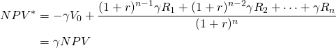
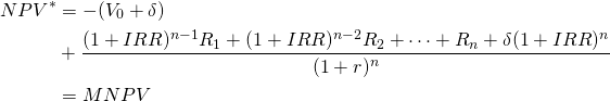
Model 1. We write the adjusted IRR* and NPV* model 1 as:
(adjusted IRR model 1)
(IRR 1)
(adjusted NPV model 1)
(NPV 1)
Model 2. We write the adjusted IRR and NPV as:
(adjusted IRR model 2)
(IRR 2)

(adjusted NPV model 2)
(NPV 2)
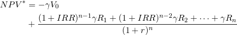
Model 3. We write the adjusted IRR* and NPV* model 3 as:
(adjusted IRR model 3)
(IRR 3)

(adjusted NPV model 3)
(NPV 3)
Model 4. We write the adjusted IRR* and NPV* model 4 as:
(adjusted IRR model 4)
(IRR 4)
(adjusted NPV model 4)
(NPV 4)
Comments on the Four Investment Models and Ranking Consistency
A comment about ranking consistency. Before commenting on models 1 through 4, we note the following. In some cases periodic and initial size-adjusted IRRs and NPVs produce the same rankings as the original IRRs and NPVs. In these cases, it simplifies our efforts to be able to use the original NPV or IRR rankings knowing they will provide the consistent rankings produced by the size adjusted IRR and NPV models.
Comments on model 1.
Notice that we can factor out the scaling factor in NPV model 1
producing the original NPV multiplied by the scaling
factor— NPV.
Moreover, ranking investments by NPV
provides the same ranking as size adjusted IRRs and NPVs. So, if
ranking needs to occur under conditions consistent with model 1,
our recommendation is to rank challengers using NPV.
NPV.
Moreover, ranking investments by NPV
provides the same ranking as size adjusted IRRs and NPVs. So, if
ranking needs to occur under conditions consistent with model 1,
our recommendation is to rank challengers using NPV.
Comments on model 2. Notice that the scaling factor in IRR model 1 cancels so that we are left with our original IRR model except that periodic cash flow are reinvested until the last period. But, compounding and discounting by the same term are offsetting actions. As a result, the IRR rankings provides the same ranking as the adjusted IRR model. So, if ranking needs to occur under conditions consistent with model 2, our recommendation is rank challengers using their original IRRs.
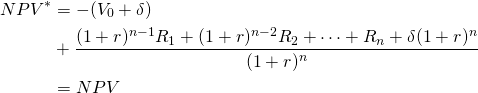
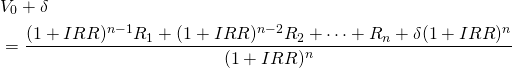
Comments on model 3.
Notice that compounding and discounting by the factor (1 +
r) in model 3 are offsetting actions so that the
adjustment produces the original NPV model except for the added
factor
that is added at the beginning and subtracted at the end of the
period—eliminating it’s influence in the model. As a result, the
original IRR rankings are the same as the size adjusted IRR and NPV
models. So, if ranking needs to occur under conditions consistent
with model three, our recommendation is rank challengers using
their original IRRs.
Comments on model 4.
Notice that compounding and discounting using the challenger’s IRR
are offsetting actions so that the adjustment produces the original
IRR model except for the added factor .
However,
is added at the beginning and subtracted at the end of the period
eliminating it from the model. As a result, the IRR rankings are
the same rankings provided by the size adjusted IRR and NPV models.
So, if ranking needs to occur under conditions consistent with
model four, our recommendation is rank challengers using their
original IRRs.
Other size adjustment models. For completeness, it is important to note that there are a number of other size adjustment methods we could employ. For example, we could combine challengers 1 and 2 in Table 9.1 to achieve initial size consistency with challenger 3. Or we could use some combination of scaling and addition to adjust for initial size differences. And the alternative reinvestment rates we could employ to resolve periodic size differences is large indeed. The only consideration when employing these nonstandard size adjustments is that the recommendations included in comments for models one through four no longer apply, requiring decision makers to find size adjusted NPVs or IRRs.
When to Rank Challengers Using Four Models
Adjusting initial investment sizes: scaling versus addition. The appropriate initial size adjustment method depends on the characteristics of the challengers in which investments are made. To compare challengers of different initial sizes, scaling to achieve initial size differences is appropriate when the challengers are available in continuous sizes or approximately so. We describe such investments as producing constant returns to scale. For constant returns to scale, the relationship between the investment and the cash flow it produces is constant. To illustrate, hours of services may often be purchased in divisible units, each unit producing the same output as earlier ones. In sum, models 1 and 2 apply when the investments are models available in continuous sizes.
On the other hand, some investments are available only in a few sizes. Machinery is available in a limited number of sizes. Sometimes, land may be purchased in fixed quantities depending on physical configurations. The same is true for buildings. So how do we compare investments available in a few sizes?
Suppose we are comparing two investments of different sizes. Assume we find the difference in their initial cost and ask: if the smaller challenger is adopted, where is the difference in their initial cost employed and what does it earn? The answer is it remains invested in the defender and these must be included with the earnings of the smaller challenger. In this way we achieve initial size consistency while allowing the underlying investments to be different in their initial sizes.
Adjusting periodic size differences: reinvestment rate assumptions. We resolved periodic size differences by setting cash flow in all of the periods to zero except cash flow in the last period. We set all of the cash flow in all but the last period equal to zero by reinvesting them. The implicit reinvestment rate for NPV and IRR models is the defender’s or the challengers’ IRRs.
Ranking Investments when the Challengers are not Mutually Exclusive
So far we have treated our challengers as mutually exclusive investments—only one can be chosen. For firms with a fixed investment budget, treating investments as mutually exclusive may be justified. Suppose that we face a set of challenging investments that are not mutually exclusive and their adoption depends on their passing some IRR hurdle. How should the investment problem be analyzed? In other words, suppose that we have a portfolio of different investment challengers and of different sizes. How big or how many challengers should be adopted ?
Economic theory can help us answer this question. Usually we array our challengers according to their IRRs and invest in the most profitable ones first. Of course, the size of the defender must match the size of the challenger, but the criterion for arranging defenders to match the size of our challenger is somewhat different. We give up, sacrifice, the defender with the smallest IRR first. To assume that defenders are infinitely scalable is to believe that the firm is in a perfect market, an assumption we earlier rejected.
Of course, investments may not come in infinitely small amounts; one large investment may be more profitable than a small investment because it is larger. If challengers come in lumpy amounts, that is the size of the challenger we investigate.
So, we are back to the place we started. Begin with the highest rate of return challenger, and sacrifice the lowest rate of return defender. Then analyze the next highest rate of return challenger and sacrifice the next lowest rate of return defender, all the time maintaining size equality. Keep analyzing challengers and defenders sequentially, maintaining size homogeneity, until you fail to adopt the next highest rate of return challenger compared to the next lowest rate of return defender.
This rule is comparable to the marginal cost equals marginal return rule employed in comparative economic static analysis.
The logic behind this arrangement is that we begin by considering the most favorable challenger, and compare it with the least favorable defender. Then we continue to the next most favorable challenger and second least favorable defender. Once we have found a challenger unable to earn a higher IRR than the IRR of the defender being sacrificed, we end our investment analysis.
Common Practice, Common Problems, and Reinvestment Rates
Common practice is to rank challengers using IRR or NPV methods. We have emphasized that this common practice can frequently produce a common problem of inconsistent rankings. Then we made the point that when challengers were adjusted for initial and periodic size differences and employed a common reinvestment rate—either the defender or the challengers’ IRRs—then the ranking were consistent. The question is, can consistent IRR and NPV rankings be achieved under fewer restrictions? For example, could we relax the common reinvestment rate assumption and still find consistent rankings—all the time? The answer is no!
Since we require only one counter-example to disprove the general claim, we provided one in Table 9.2. Consider three challengers of equal initial size and different periodic cash flow. Since reinvesting the cash flow to achieve periodic size equality at the defender’s IRR doesn’t change NPV rankings and reinvesting at the challenger’s IRR doesn’t change IRR rankings, we can rank the three challengers using NPV and IRR under initial and periodic size equality. We reported the results of such a comparison earlier in Table 9.2.
Note the conflicting NPV and IRR rankings. NPV ranks the three challengers 1, 2, and 3. IRR ranks the three challengers 3, 1, and 2. These results provide the one counter example needed to disprove the claim that different reinvestment rates are not required for consistent rankings. Furthermore, since we are describing the reinvestment rate for the same investment and are only changing the ranking method, consistency would require the same reinvestment rate assumption regardless of the ranking method employed.
Summary and Conclusions
This chapter has demonstrated that equal initial investments and periodic cash flows reinvested until the last period plus a common reinvestment rate across IRR and NPV models are sufficient conditions for consistent MIRR and MNPV investment rankings. We can make unequal initial investments equal by scaling or adding investments to the small challengers—and by some other methods, if required. Whether or not initial size differences are resolved by scaling or by addition depends on whether the challenger is available in continuous sizes in which case scaling is appropriate. Otherwise, if it is unique and cannot be scaled, size differences are resolved by additions. All other methods for resolving initial size differences ultimately create additional challengers.
Resolving periodic size differences required that we reinvest cash flow until the final period. We considered the defender’s IRR and the challengers’ IRRs as possible reinvestment rates. Of course, there are a number of other possible reinvestment rate choices. The important point is that if the discount rate and the reinvestment rate are different, then the NPV rankings will be stable and will not vary with the discount rate.
Questions
- Discuss why some investment analysts prefer NPV methods to rank investments while others prefer IRR methods. Which do you prefer? Defend your answer.
- Provide three reasons why NPV and IRR rankings may be inconsistent.
- Refer to the investment problems described in Table Q9.1 below. Notice that initial investment sizes are unequal as are the periodic cash flows in period one which produce the inconsistent NPV and IRR ranking reported in the last two columns and rows of Table Q9.1. We will refer to the results in Table Q9.1 in several questions that follow.
Table Q9.1. NPVs and IRRs for two mutually exclusive investments assuming a discount rate equal to the defender’s IRR of r = 5%.
| initial investments
where i = 1,2 |
period one cash flows
where t = 1 generated by initial investments
where i = 1,2 |
period two cash flows
where t = 2 generated by initial investments
where i = 1,2 |
NPVi earned by initial investments
where i = 1,2 assuming r = 5% (ranking) |
IRRi earned by initial investments
where i = 1,2 (ranking) |
 |
$2,000 | $1,500 | $265.31 (1) |
11.51% (2) |
 |
$800 | $400 | $124.72 (2) |
14.83% (1) |
-
- Complete Table Q9.2 by finding MNPVs and MIRRs for the two investments assuming a discount rate and reinvestment rate equal to the defender’s IRR, of r=5%. Include the investment rankings in the parentheses.
Table Q9.2. MNPVs and MIRRs for two mutually exclusive investments assuming a discount and reinvestment rate of r = 5%.
| initial investments
where i = 1,2 |
period one cash flows
where t = 1 generated by initial investments
where i = 1,2 |
period two cash flows
where t = 2 generated by initial investments
where i = 1,2 |
MNPVi
earned by initial investments
where i = 1,2 assuming r = 5% (ranking) |
MIRRi
earned by initial investments
where i = 1,2 assuming r = 5% (ranking) |
 |
$1,500 + $2,000(1.05) = $3,600 | $ ( ) |
% ( ) |
|
 |
$400 + $800(1.05) = $1,240 | $ ( ) |
% ( ) |
-
- Complete Table Q9.3 by finding MNPVs and MIRRs for the two investments assuming a discount rate and reinvestment rate equal to the defender’s IRR, of r = 5% and a reinvestment rates equal to the investments’ IRRs. Include the investment rankings in the parentheses.
Table Q9.3. MNPVs and MIRRs for two mutually exclusive investments assuming a discount and reinvestment rate of r = 5%. and reinvestment rates equal to the investments’ IRRs
| initial investments
where i = 1,2 |
period one cash flows
where t = 1 generated by initial investments
where i = 1,2 |
period two cash flows
where t = 2 generated by initial investments
where i = 1,2 |
MNPVi earned by initial investments
where i = 1,2 assuming the discount and reinvestment rate
equal r = 5% (ranking) |
MIRRi earned by initial investments
where i = 1,2 assuming the reinvestment rate equals
r = 5% (ranking) |
|
$1,500 + $2,000(1.1151) = $3,730.20 | $ ( ) |
% ( ) |
|
|
$400 + $800(1.1483) = $1,318.64 | $ ( ) |
% ( ) |
-
- Complete Table Q9.4 by finding scaled MNPVs and scaled MIRRs for the two investments assuming a discount rate and reinvestment rate equal to the defender’s IRR, of r=5%. What is the scaling factor you are using? Include the investment rankings in the parentheses.
Table Q9.4. Scaled MNPVs and MIRRs for two mutually exclusive investments assuming a discount and reinvestment rate of r = 5%.
initial investment  where i = 1,2
 |
period one cash flows  where t = 1 generated by initial investments
where i = 1,2
where t = 1 generated by initial investments
where i = 1,2 |
period two cash flows
where t = 2 generated by initial investments
where i = 1,2 |
Scaled MNPVi earned by scaled initial
investments
where i = 1,2 assuming the discount and reinvestment rate
equal r = 5% (ranking) |
Scaled MIRRs earned by scaled initial investments
where i = 1,2 assuming the discount and reinvestment rate
equal r = 5% (ranking) |
 |
$1,500 + [$2,000(1.05)] = $3,600 | $ ( ) |
% ( ) |
|
|
[(3)$400] + [(3)$800(1.05)] = $3,720 | $ ( ) |
% ( ) |

-
- Complete Table Q9.5 by finding scaled MNPVs and scaled MIRRs for the two investments assuming a discount rate equal to the defender’s IRR, of r = 5% and reinvestment rates equal to the investments’ IRRs. Include the investment rankings in the parentheses.
Table Q9.5. Scaled MNPVs and MIRRs for two mutually exclusive investments assuming a discount rate of r = 5% and reinvestment rates equal to the investments’ IRRs
| initial investment
where i = 1,2 |
period one cash flows
where t = 1 generated by initial investments
where i = 1,2 |
period two cash flows
where t = 2 generated by initial investments
where i = 1,2 |
Scaled MNPVi earned by scaled initial
investments
where i = 1,2 assuming the discount rate r = 5%
and reinvestment rates equal to the investments’ IRRs
(rankings) |
Scaled MIRRs earned by scaled initial investments
where i = 1,2 assuming the reinvestment rate equals r = 5%
(ranking) |
|
$1,500 + [$2,000(1.1151)] = $3,730.20 | $ ( ) |
% ( ) |
|
|
|
[(3)$400] + [(3)$800(1.1483)] = $3,955.92 | $ ( ) |
% ( ) |
-
- Complete Table Q9.6 by finding added MNPVs and MIRRs for the
two investments assuming a discount and reinvestment rate equal to
the defender’s IRR, of r = 5%. What is the additional
investment amount
added to the smaller investment? Include the investment rankings in
the parentheses.
- Complete Table Q9.6 by finding added MNPVs and MIRRs for the
two investments assuming a discount and reinvestment rate equal to
the defender’s IRR, of r = 5%. What is the additional
investment amount
Table Q9.6. Added MNPVs and MIRRs for two mutually exclusive investments assuming a discount rate of r = 5% and reinvestment rates equal to the defender’s IRR of r = 5%.
Initial plus added
investments  where i = 1,2
 |
period one cash flows
where t = 1 generated by initial plus added investments
where i=1,2 |
period two cash flows
 where t=2 generated by initial plus added investment
where i = 1,2
where t=2 generated by initial plus added investment
where i = 1,2 |
Added
MNPVi earned by initial plus added investments
where i = 1,2 assuming the discount rate and reinvestment
rate r = 5% (rankings) |
Added
MIRRi where i = 1,2 earned by initial
plus added investments
where i = 1,2 assuming the reinvestment rate r =
5% (rankings) |
|
$1,500 + $2,000(1.05) = $3,600 | $ ( ) |
% ( ) |
|
 where
where  |
$400 + $800(1.05) + $2,000(1.05)2 = $3,445 | $ ( ) |
% ( ) |
-
- Complete Table Q9.7 by finding added MNPVs and MIRRs for the two investments assuming a discount rate equal to the defender’s IRR, of r = 5% and reinvestment rates equal to the investments’ IRRs. Include the investment rankings in the parentheses.
Table Q9.7. Added MNPVs and MIRRs for two mutually exclusive investments assuming a discount rate of r = 5% and reinvestment rates equal to the investments’ IRRs
| Initial plus added
investments
where i = 1,2 |
period one cash flows
where t = 1 generated by initial plus added investments
where i=1,2 |
period two cash flows
where t=2 generated by initial plus added investment
where i = 1,2 |
Added
MNPVi earned by initial plus added investments
where i = 1,2 assuming the discount rate r = 5%
and reinvestment rates equal to the investments’ IRRs
(rankings) |
Added
MIRRi earned by initial plus added investments
where i = 1,2 assuming the reinvestment rate r =
5% (rankings) |
|
$1,500 + [$2,000(1.1151)] = $3,730.20 | $ ( ) |
% ( ) |
|
|
where |
$400 + [$800(1.1483)] + $2,000(1.1483)2 = $3,955.83 | $ ( ) |
% ( ) |
- To answer the questions that follow, first complete Table Q9.8 using data from the completed Tables in question 3. Cells indicated with an “n.a.” do not require an answer.
Table Q9.8. Summary of rankings described in Tables Q9.1 through Q9.7
| Table provide the data | Type of ranking | Assuming reinvestment rate is defender’s IRR | Assuming reinvestment rate is investments IRR | ||
| Investment 1 | Investment 2 | Investment 1 | Investment 2 | ||
| Q9.1 | NPV | n.a. | n.a. | ||
| IRR | n.a. | n.a. | |||
| Q9.2 | MNPV | n.a. | n.a. | ||
| MIRR | n.a. | n.a. | |||
| Q9.3 | MNPV | n.a. | n.a. | ||
| MIRR | n.a. | n.a. | |||
| Q9.4 | Scaled MNPV | n.a. | n.a. | ||
| Scaled MIRR | n.a. | n.a. | |||
| Q9.5 | Scaled MNPV | n.a. | n.a. | ||
| Scaled MIRR | n.a. | n.a. | |||
| Q9.6 | Added MNPV | n.a. | n.a. | ||
| Added MIRR | n.a. | n.a. | |||
| Q9.7 | Added MNPV | n.a. | n.a. | ||
| Added MIRR | n.a. | n.a. | |||
-
- Referring to your completed Table Q9.8, which ranking methods produce consistent results? Please explain your answer.
- Referring to your completed Table Q9.8, which consistent ranking method(s) are consistent with NPV rankings? Please explain your answer.
- Referring to your completed Table Q9.8, which consistent ranking method(s) are consistent with scaled NPVs? Please explain your answers.
- Referring to your completed Table Q9.8, which consistent ranking method(s) are consistent with IRRs? Please explain your answers.
- Explain why investments of unequal term can be examined using the ranking methods described in this chapter.
- Much of the material in this chapter was published in Robison, Myers, and Barry (2015). ↵