
5.1: Interest Rate Fluctuations
- Page ID
- 569
- As a first approximation, what causes the interest rate to change?
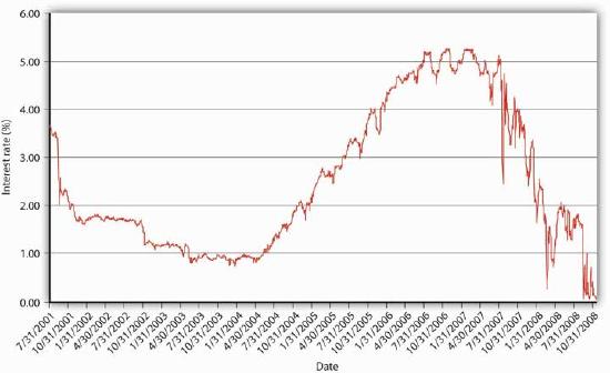
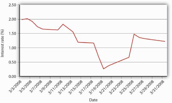
If you followed the gist of Chapter 4, you learned (we hope!) about the time value of money, including how to calculate future value (FV), present value (PV), yield to maturity, current yield (the yield to maturity of a perpetuity), rate of return, and real interest rates. You also learned that a change in the interest rate has a profound effect on the value of assets, especially bonds and other types of loans, but also equities and derivatives. (In this chapter, we’ll use the generic term bonds throughout.) That might not be a very important insight if interest rates were stable for long periods. The fact is, however, interest rates change monthly, weekly, daily, and even, in some markets, by the nanosecond. Consider Figure 5.1 and Figure 5.2. The first figure shows yields on one-month U.S. Treasury bills from 2001 to 2008, the second shows a zoomed-in view on just March 2008. Clearly, there are long-term secular trends as well as short-term ups and downs.
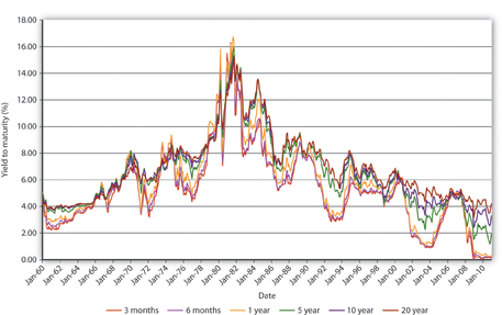
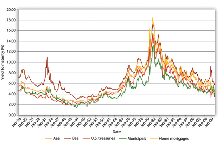
You should now be primed to ask, Why does the interest rate fluctuate? In other words, what causes interest rate movements like those shown above? In this aptly named chapter, we will examine the economic factors that determine the nominal interest rate. We will ignore, until the next chapter, the fact that interest rates differ on different types of securities. In this chapter we will concern ourselves only with the general level of interest rates, which economists call “the” interest rate. As Figure 5.3 and Figure 5.4 show, interest rates tend to track each other, so by focusing on what makes one interest rate move, we have a leg up on making sense of movements in the literally thousands of interest rates out there in the real world.

The ability to forecast changes in the interest rate is a rare but profitable gift. Professional interest rate forecasters are seldom right on the mark and often are far astray, and half the time they don’t even get the direction (up or down) right.[1] That’s what we’d expect if their forecasts were determined by flipping a coin! Therefore, we don’t expect you to be able to predict changes in the interest rate, but we do expect you to be able to post-dict them. In other words, you should be able to narrate, in words and appropriate graphs, why past changes occurred. You should also be able to make predictions by invoking the ceteris paribus assumption.
The previous graphs reveal that interest rates generally trended downward from 1920 to 1945, then generally rose until the early 1980s, when they began trending downward again through 2011. During the 1920s, general business conditions were favorable. In other words, taxes and regulations were relatively low, while confidence in public policies was high. President Calvin Coolidge summed this up when he said, “The business of America is business.” Therefore, the demand for bonds increased (the demand curve shifted right), pushing prices higher and yields lower. The 1930s witnessed the Great Depression, an economic recession of unprecedented magnitude that dried up profit opportunities for businesses and hence shifted the supply curve of bonds hard left, further increasing bond prices and depressing yields. (If the federal government had not run budget deficits some years during the depression, the interest rate would have dropped even further.) During World War II, the government used monetary policy to keep interest rates low. After the war, that policy came home to roost as inflation began to become, for the first time in American history, a perennial fact of life. Contemporaries called it “creeping inflation.” A higher price level, of course, put upward pressure on the interest rate (think Fisher Equation). The unprecedented increase in prices during the 1970s (what some have called the “Great Inflation”) drove nominal interest rates higher still. Only in the early 1980s, after the Federal Reserve mended its ways (a topic to which we will return) and brought inflation under control, did the interest rate begin to fall. Positive geopolitical events in the late 1980s and early 1990s, namely, the end of the Cold War and the birth of what we today call “globalization,” also helped to reduce interest rates by rendering the general business climate more favorable (thus pushing the demand curve for bonds to the right, bond prices upward, and yields downward). Pretty darn neat, eh?
The keys to understanding why “the” interest rate changes over time are simple price theory (supply and demand) and the theory of asset demand. Like other types of goods, bonds and other financial instruments trade in markets. The demand curve for bonds, as for most goods, slopes downward; the supply curve slopes upward in the usual fashion. There is little mystery here. The supply curve slopes upward because, as the price of bonds increases (which is to say, as their yield to maturity decreases), holding the bonds’ face values and coupons and the rest of the world constant, borrowers (sellers of securities) will supply a higher quantity, just as producers facing higher prices for their wares will supply more cheese or automobiles. As the price of bonds falls, or as the yield to maturity that sellers and borrowers offer increases, sellers and borrowers will supply fewer bonds. (Why sell ’em if they aren’t going to fetch much?) When they can obtain funds cheaply, companies will be eager to borrow to expand because it is more likely that it will be profitable to do so. When funds are dear, companies will not see many positive present net value projects to pursue.
The demand curve for bonds slopes downward for similar reasons. When bond prices are high (yields to maturity are low), few will be demanded because investors (buyers) will find other, more lucrative uses of their money. As bond prices fall (bond yields increase), investors will want more of the increasingly good deals (better returns) that they offer.
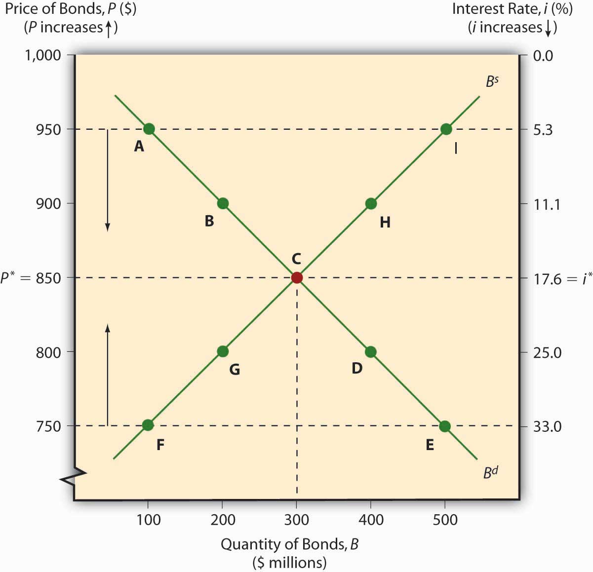
The market price of a bond and the quantity that will be traded is determined, of course, by the intersection of the supply and demand curves, as in Figure 5.5. The equilibrium price prevails in the market because, if the market price were temporarily greater than p*, the market would be glutted with bonds. In other words, the quantity of bonds supplied would exceed the quantity demanded, so sellers of bonds would lower their asking price until equilibrium was restored. If the market price temporarily dipped below p*, excess demand would prevail (the quantity demanded would exceed the quantity supplied), and investors would bid up the price of the bonds to the equilibrium point.
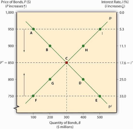
As with other goods, the supply and demand curves for bonds can shift right or left, with results familiar to principles (“Econ 101”) students. If the supply of bonds increases (the supply curve shifts right), the market price will decrease (the interest rate will increase) and the quantity of bonds traded will increase. If the supply of bonds decreases (the supply curve shifts left), bond prices increase (the interest rate falls) and the equilibrium quantity decreases. If the demand for bonds falls (the demand curve shifts left), prices and quantities decrease (and the interest rate increases). If demand increases (the demand curve shifts right), prices and quantities rise (and the interest rate falls).
- The interest rate changes due to changes in supply and demand for bonds.
- Or, to be more precise, any changes in the slopes or locations of the supply and/or demand curves for bonds (and other financial instruments) lead to changes in the equilibrium point (p* and q*) where the supply and demand curves intersect, which is to say, where the quantity demanded equals the quantity supplied.