
11.3: Short Term Business Decisions
- Page ID
- 26124
Project selection: Payback period
The payback period is the time it takes for the cumulative sum of the annual net cash inflows from a project to equal the initial net cash outlay. In effect, the payback period answers the question: How long will it take the capital project to recover, or pay back, the initial investment?
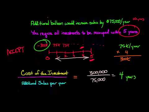
A YouTube element has been excluded from this version of the text. You can view it online here: pb.libretexts.org/llmanagerialaccounting/?p=246
If the net cash inflows each year are a constant amount, the formula for the payback period is:
| Payback period = | Initial cash outlay |
| Annual net cash inflow (benefit) |
For the two assets discussed in the previous section, you can compute the payback period as follows. The purchase of the $120,000 equipment creates an annual net cash inflow after taxes of $18,200, so the payback period is 6.6 years, computed as follows:
| Payback period = | Initial cash outlay | = 120,000 | = 6.6 years (rounded) |
| Annual net cash inflow (benefit) | 18,200 |
The payback period for the replacement machine with a $28,000 cash outflow in the first year and an annual net cash inflow of $2,600, is 10.8 years, computed as follows:
| Payback period = | Initial cash outlay | = 28,000 | = 10.8 years (rounded) |
| Annual net cash inflow (benefit) | 2,600 |
Remember that the payback period indicates how long it will take the machine to pay for itself. The replacement machine being considered has a payback period of 10.8 years but a useful life of only 8 years. Therefore, because the investment cannot pay for itself within its useful life, the company should not purchase a new machine to replace the two old machines.
In each of the previous examples, the projected net cash inflow per year was uniform. When the annual returns are uneven, companies use a cumulative calculation to determine the payback period, as shown in the following situation.
Neil Company is considering a capital investment project that costs $40,000 and is expected to last 10 years. The projected annual net cash inflows are:
| Year | Investment | Annual net cash inflow | Cumulative net cash inflows |
| 0 | $ 40,000 | —– | — |
| 1 | — | $ 8,00 | $ 8,000 |
| 2 | — | 6,000 | 14,000 |
| 3 | — | 7,000 | 21,000 |
| 4 | —- | 5,000 | 26,000 |
| 5 | — | 8,000 | 34,000 |
| 6 | — | 6,000 | 40,000 |
| 7 | — | 3,000 | 43,000 |
| 8 | — | 2,000 | 45,000 |
| 10 | — | 1,000 | 49,000 |
The payback period in this example is six years, the time it takes to recover the $40,000 original investment as show in the cumulative net cash inflows of year 6.
When using payback period analysis to evaluate investment proposals, management may choose one of these rules to decide on project selection:
- Select the investments with the shortest payback periods.
- Select only those investments that have a payback period of less than a specified number of years.
Both decision rules focus on the rapid return of invested capital. If capital can be recovered rapidly, a firm can invest it in other projects, thereby generating more cash inflows or profits.
Some managers use payback period analysis in capital budgeting decisions due to its simplicity. However, this type of analysis has two important limitations:
- Payback period analysis ignores the time period beyond the payback period. For example, assume Allen Company is considering two alternative investments; each requires an initial outlay of $30,000. Proposal Y returns $6,000 per year for five years, while proposal Z returns $5,000 per year for eight years. The payback period for Y is five years ($30,000/$6,000) and for Z is six years ($30,000/$5,000). But, if the goal is to maximize income, proposal Z should be selected rather than proposal Y, even though Z has a longer payback period. This is because Z returns a total of $40,000 ($5,000 per year x 8 years), while Y simply recovers the initial $30,000 ($6,000 per year for 5 years) outlay.
- Payback analysis also ignores the time value of money. For example, assume the following net cash inflows are expected in the first three years from two capital projects:
| Net Cash Inflows | ||
| Project A | Project B | |
| First year | $ 15,000 | $ 9,000 |
| Second year | 12,000 | 12,000 |
| Third year | 9,000 | 15,000 |
| Total | $ 36,000 | $ 36,000 |
Assume that both projects have the same net cash inflow each year beyond the third year. If the cost of each project is $36,000, each has a payback period of three years. But common sense indicates that the projects are not equal because money has time value and can be reinvested to increase income. Because larger amounts of cash are received earlier under Project A, it is the preferable project.
Project selection: Unadjusted rate of return or Accounting rate of return
Another method of evaluating investment projects that you are likely to encounter in practice is the accounting (or unadjusted) rate of return method. To compute the accounting rate of return, you will need to know 2 things:
- Annual income after taxes; and
- Average amount of the investment in the project. The average investment is the (Beginning balance + Ending balance)/2. If the ending balance is zero (as we assume), the average investment equals the original cash investment divided by 2.
The formula for the unadjusted (or Accounting) rate of return is:
| Rate of Return = | Average annual income after taxes |
| Average amount of investment |
Notice that this calculation uses annual income rather than net cash inflow.[1]

A YouTube element has been excluded from this version of the text. You can view it online here: pb.libretexts.org/llmanagerialaccounting/?p=246
To illustrate the use of the unadjusted rate of return, assume Thomas Company is considering two capital project proposals, each having a useful life of three years. The company does not have enough funds to undertake both projects. Information relating to the projects follows:
| Average annual Before-tax | Average | |||
| Proposal | Initial cost | Salvage Value | Net cash inflow | Annual depreciation |
| 1 | $ 76,000 | $ 4,000 | $ 45,000 | $ 24,000 |
| 2 | 95,000 | 5,000 | 55,000 | 30,000 |
Assuming a 40% tax rate, Thomas Company can determine the unadjusted rate of return for each project as follows:
| Proposal 1 | Proposal 2 | ||
| Average investment: (original outlay + Salvage value)/2 | (1) | $ 40,000 | $ 50,000 |
| (76,000 + 4,000) / 2 | (95,000 + 5,000) / 2 | ||
| Annual net cash inflow (before income taxes) | $ 45,000 | $ 55,000 | |
| Less: Annual depreciation | – 24,000 | – 30,000 | |
| Annual income (before income taxes) | $ 21,000 | $ 25,000 | |
| Deduct: Income taxes at 40% | – 8,400 | – 10,000 | |
| Average annual net income from investment | (2) | $ 12,600 | $ 15,000 |
| Rate of return (2)/(1) | 31.5% | 30% | |
| (12,600 / 40,000) | (15,000 / 50,000) |
From these calculations, if Thomas Company makes an investment decision solely on the basis of the unadjusted rate of return, it would select Proposal 1 since it has a higher rate.
Sometimes companies receive information on the average annual after-tax net cash inflow. Average annual after-tax net cash inflow is equal to annual before-tax cash inflow minus taxes. Given this information, the firms could deduct the depreciation to arrive at average net income. For instance, for Proposal 2, Thomas Company would compute average net income as follows:
| After-tax net cash inflow ($55,000-$10,000) | $ 45,000 |
| Less: Depreciation | – 30,000 |
| Average net income | $ 15,000 |
The unadjusted rate of return, like payback period analysis, has several limitations:
- The length of time over which the return is earned is not considered.
- The rate allows a sunk cost, depreciation, to enter into the calculation. Since depreciation can be calculated in so many different ways, the rate of return can be manipulated by simply changing the method of depreciation used for the project.
- The timing of cash flows is not considered. Thus, the time value of money is ignored.
Unlike the two project selection methods just illustrated, the remaining two methods—net present value and time-adjusted rate of return—take into account the time value of money in the analysis. In both of these methods, we assume that all net cash inflows occur at the end of the year. Often used in capital budgeting analysis, this assumption makes the calculation of present values less complicated than if we assume the cash flows occurred at some other time.
- Accounting Principles: A Business Perspective.. Authored by: James Don Edwards, University of Georgia & Roger H. Hermanson, Georgia State University.. Provided by: Endeavour International Corporation. Project: The Global Text Project. License: CC BY: Attribution
- The Payback Method. Authored by: Education Unlocked. Located at: youtu.be/YX4NoZN8YWU. License: All Rights Reserved. License Terms: Stanard YouTube License
- Average Accounting Rate of Return CFA-Course.com . Authored by: cfa-course.com. Located at: youtu.be/-E5Z1-0NUmk. License: All Rights Reserved. License Terms: Standard YouTube License